Now that we understand the architecture of the Origin2000 system, it is time to address "tuning," i.e., how do we get our programs to run fast on this architecture?
We can break tuning into 5 steps:
Just as in tuning, we'll now take things one step at a time.
If you don't have to get the right answer, you can make a program run arbitrarily fast, so the very first rule in tuning is that the program has to generate the correct results. While this may seem obvious, it is quite easy to forget to check the answers along the way as one is making performance improvements. A lot of frustration can be avoided by making only one change at a time and verifying that the program is still correct after each change.
In addition to problems introduced by performance changes, correctness issues may be raised simply in porting a code from one system to another. If the program is written in a high level language and adheres to the language standard, it will generally port with no difficulties. This is particularly true for standard-compliant Fortran-77 programs, but there are some exceptions for C programs.
Irix 6.x is a 64-bit operating system. While programs may be compiled and run as if it were a 32-bit operating system, you often want to take advantage of the larger address space and compile in 64-bit mode. In this mode, both pointers and long integers are 64 bits in size, while int's remain 32 bits. If a program assumes that pointers and int's are both 32 bits long, run-time faults and/or incorrect answers can result. If this occurs, there are two remedies: either correct the program so that types of different sizes are not haphazardly intermixed, or ignore the coding problems and compile the program to run in 32-bit mode. The second solution is certainly expedient, and is even a perfectly reasonable approach for programs which will never grow beyond the confines of a 32-bit address space. But if one wishes a program to be able to exploit the advantages of the 64-bit operating system, correcting the size problems is the proper solution.
One selects which mode to compile in via the flags -32, -n32 and -64. The "mode" is more often called the ABI, or Application Binary Interface (see abi(5) for a detailed explanation of ABIs). -32 is the default ABI since it provides the highest level of portability.
However, programs compiled using this ABI not only cannot take advantage
of many of the extra capabilities of the 64-bit operating system, they also
are limited to the MIPS I and MIPS II instruction sets. If one wishes to
use the capabilities of the MIPS III or MIPS IV instructions sets, then
one needs to compile with either -n32 or -64.
With the -n32 ABI, pointers and long ints are still 32 bits in size, so one retains the
portability of the -32 ABI. -n32 differs from -32 in that instead of generating programs with just the MIPS I or MIPS II ISAs, it allows programs to be generated using either the MIPS III or MIPS
IV ISAs, as selected by the -mips3 and -mips4 flags, respectively. With the -64 flag, pointers and long ints are 64 bits in length, so full advantage may
be taken of the 64-bit operating system. As with -n32, either the MIPS III or MIPS IV ISAs may be chosen.
On Origin2000 (and all other non-R8000) systems, the default ABI and ISA
are -32 -mips2; on R8000-based systems, the defaults are -64 -mips4. Because the defaults vary by system type, it is highly recommended that
the desired ABI and ISA be explicitly declared for each compilation. The
clearest way to do this is to specify these options directly in a makefile
(see make(1) and pmake(1)) so they are used by all compilation commands:
ABI     = -n32
ISA     = -mips4
CFLAGS  = $(ABI) $(ISA) -Ofast

        .
        .
        .

.c.o:
        $(CC) $(CFLAGS) -c $<
An alternative approach is to to make use of a defaults specification file. This is a file which tells the compiler which ABI and ISA it should use if none have been specified in the compilation command. The system adminstrator may create the file /etc/compiler.defaults to set the defaults for a particular system. Individual users may create their own compiler.defaults files and then tell the compiler where to look for them by setting the environment variable COMPILER_DEFAULTS_PATH; the first such file found in this colon-separated path list will take precedence over the system-wide file. If a default specification file has been provided, its contents will override the compiler's built-in defaults (but not the options specified explicitly in the compilation command).
The contents of the compiler.defaults file must be the the following specifier:
-DEFAULT:[abi={32|n32|64}]:[isa={mips1|mips2|mips3|mips4}]:[proc={r4k|r5k|r8k|r10k}]
which allows one to indicate the default ABI and ISA, as well as which processor to compile for (more on this option later).
One final method is available for specifying the ABI. One can set the environment variable SGI_ABI to -32, -n32 or -64 to specify the default ABI. If this environment variable is set, it will override the setting in the defaults specification file; a command line setting, however, will take precedence over this environment variable.
Unless it is a requirement that the binary can be run on an R4000-based system (which supports MIPS III, but not MIPS IV), use one of the following ABI/ISA combinations
% cc -64 -mips4 ...
% cc -n32 -mips4 ...
for C, and similarly for the other languages. The same ABI (but not necessarily ISA) must be used for all objects comprising a single executable. Different executables may use different ABIs, however. For more information on these compiler flags, as well as the defaults specification file, see the man pages for cc(1), f77(1), CC(1), f90(1), ld(1).
A program can fail to port for other reasons. Since different compilers handle standards violations differently, non-standard-compliant programs often generate different results when rehosted. An often seen example of this is a Fortran program which assumes that all variables are initialized to 0. While this initialization occurred on most older machines, it is not done in general on newer, stack-based architectures. When a program making such an assumption is rehosted to a new machine, it will almost certainly generate incorrect results.
To detect this error, one can compile with the -trapuv flag. This flag initializes all unitialized variables in a program with the value 0xFFFA5A5A. When this value is used as a floating point variable, it is treated as a floating point NaN and it will cause a floating point trap. When it is used as a pointer, an address or segmentation violation will most likely occur. By running the program with a debugger, such as dbx(1), the use of such an uninitialized variable can be pinpointed, and the program can then be fixed to do the proper initialization.
While fixing the program is the "right thing to do," it does require some
effort by the programmer. An alternative, which requires almost no effort,
is to use the -static flag. This flag causes all variables to be allocated from a static data
area rather than the stack, and these variables will then be initialized
to 0. There is a cost to the easy way out, however. Use of the -static flag generally hurts program performance; a 20% penalty is not uncommon.
Another trick which can sometimes help in rehosting a program is to compile
with the lowest optimization level, -O0 (i.e., no optimization), but this, too will significantly hurt performance.
Other types of porting failures can occur as well. The results generated on one computer may disagree with those from another computer because of differences in the floating point format, or compiler differences which cause the roundoff error to change. One needs to understand the particular program in order to determine if these differences are significant. In addition, some programs may fail to even compile on a new system if extensions are not supported or are provided with a different syntax; Fortran pointers provide a good example of this. In such situations, the code must be modified to be compatible with the new compiler. Similarly, if a program makes calls to a particular vendor's libraries, these calls will need to be replaced with equivalent entry points from the new vendor's libraries.
Finally, programs sometimes have mistakes in them which by pure luck had previously not caused problems. But when compiled on a new system, errors finally appear. Writing beyond the end of an array can show this behavior. Such mistakes need to be corrected. For f77 compilations, one can use the -C (or, equivalently, -check_bounds) flag to instruct the Fortran compiler to generate code for runtime subscript range checking. If an out-of-bounds array reference is made, the program will abort and display an error message indicating the illegal reference which was made and which line of code it occurred on:
Subscript out of range on file line 6, procedure MAIN_.
Attempt to access the 0-th element of variable ?.
*** Execution Terminated (99) ***
When tracking down the source of incorrect results, a symbolic debugger is an invaluable tool. Two such debuggers are available for the Origin2000 system. dbx is the standard Unix debugger which has been available for many years. It uses a simple, teletype style interface and may be used to debug sequential programs or multi-processor programs, although the MP debugging is somewhat awkward. cvd, the WorkShop debugger, uses a graphical user interface and provides greater fuctionality and efficiency than dbx; it is also much more convenient for debugging multi-processor programs. For information on how to use these products, consult the dbx(1) reference page and the Developer Magic: Debugger User's Guide.
The quickest and easiest way to improve the performance of a program is to link it with libraries already tuned for the target hardware. In addition to the standard libraries, such as libc, whose hardware-specific versions are automatically linked in with programs compiled and run on the Origin2000 system, there are two other libraries which may optionally be used which can provide substantial performance benefits.
libfastm provides highly optimized versions of a subset of the routines found in libm, the standard math library. Optimized scalar versions of sin, cos, tan, exp, log, and pow for both single- and double-precision are provided. To link in libfastm, append -lfastm to the end of the link line:
cc -o program <objects> -lfastm Separate versions of libfastm exist for the R10000, R8000 and R5000. In order to link with the correct
version, the desired chip should be explicitly requested with the -r10000, -r8000 or -r5000 flags, respectively. When used on the compile line, these flags also instruct
the compiler to generate code scheduled for the specified chip. For Origin2000
systems, the -r10000 flag should be used when compiling and linking.
In addition the scalar routines just mentioned, the following vector intrinsics are now part of the standard math library: vacos, vasin, vatan, vcos, vexp, vlog, vsin, vsqrt and vtan, plus the single precision versions whose names are derived from those of these double precision versions by appending an f. This library is linked in automatically by Fortran; the -lm flag should be used when linking with ld or the C compiler:
cc -o program <objects> -lmMore information on the math intrinsics can be found in math(3M) and libfastm(3M), and an description of when the compiler will use the vector math intrinsics automatically is presented later.
complib.sgimath The other library which provides optimized code is complib.sgimath. This is a library of mathematical routines for carrying out linear algebra operations, FFTs and convolutions. It contains optimized implementations of the public domain libraries LINPACK, EISPACK, LAPACK, FFTPACK, and the Level-1, -2 and -3 BLAS, plus proprietary sparse solvers tuned specifically for Silicon Graphics, Inc. platforms.
Many of the complib routines have been parallelized, so there are separate sequential and parallel
versions of the library. To link in the sequential version of complib.sgimath, add -lcomplib.sgimath to the link line:
f77 -o program <objects> -lcomplib.sgimath -lfastm To link in the parallel version, use -lcomplib.sgimath_mp; in addition, the -mp flag must be used when linking in the parallel code:
f77 -mp -o program <objects> -lcomplib.sgimath_mp -lfastm Since complib.sgimath uses some routines found in libfastm, libfastm should be linked in after complib.sgimath.
For more information about these libraries, see the man pages for libfastm(3M), math(3M), complib(3F), blas(3F), lapack(3F), fft(3F), conv(3F), solvers(3F), psldu(3F), psldlt(3F), and pskysl(3F).
When confronted with a program composed of hundreds of modules and thousands of lines of code, it would require a very heroic, and very inefficient, effort to tune the entire program. Tuning needs to be concentrated on those few sections of the code where the work will pay off with the biggest gains in performance. These sections of code are identified with the help of a profiler.
The hardware counters in the R10000 CPU make it possible to profile the behavior of a program in many ways without modifying the code. The software tools are:
You use these tools to find out what constrains the program, and which parts of the it consume the most time. Through the use of a combination of these tools, it is possible to identify most performance problems.
The profiling tools depend for most of their features on the R10000's Performance Counter Registers. These on-chip registers can be programmed to count hardware events as they happen, for example machine cycles, instructions, branch predictions, floating point instructions, or cache misses.
There are only two Performance Counter registers. Each can be programmed to count machine cycles or one of 15 other events, for a total of 32 events that can be counted (30 of which are distinct). The specific events are summarized in the following table which can always be obtained by using the command perfex -h. A detailed discussion of the events is contained in this sidebar on counter definitions.
| Event Number | Counter 0 Event | Event Number | Counter 1 Event |
|---|---|---|---|
| 0 | Cycles | 16 | Cycles |
| 1 | Instructions issued to functional units | 17 | Instructions graduated |
| 2 | Memory data access (load, prefetch, sync, cacheop) issued | 18 | Memory data loads graduated |
| 3 | Memory stores issued | 19 | Memory data stores graduated |
| 4 | Store-conditionals issued | 20 | Store-conditionals graduated |
| 5 | Store-conditionals failed | 21 | Floating-point instructions graduated |
| 6 | Branches decoded | 22 | Quadwords written back from L1 cache |
| 7 | Quadwords written back from L2 cache | 23 | TLB refill exceptions |
| 8 | Correctable ECC errors on L2 cache | 24 | Branches mispredicted |
| 9 | L1 cache misses (instruction) | 25 | L1 cache misses (data) |
| 10 | L2 cache misses (instruction) | 26 | L2 cache misses (data) |
| 11 | L2 cache way mispredicted (instruction) | 27 | L2 cache way mispredicted (data) |
| 12 | External intervention requests | 28 | External intervention request hits in L2 cache |
| 13 | External invalidate requests | 29 | External invalidate request hits in L2 cache |
| 14 | Instructions done (formerly, virtual coherency condition) | 30 | Stores, or prefetches with store hint, to CleanExclusive L2 cache blocks |
| 15 | Instructions graduated | 31 | Stores, or prefetches with store hint, to Shared L2 cache blocks. |
The counters are 64-bit integers. When a counter overflows, a hardware trap occurs. The kernel can preload a counter with (2^64 - n) to cause a trap after n counts occur. The profiling tools use this capability. For example, the command ssrun -gi_hwc programs the graduated instruction counter (event 17) to overflow every 32K counts. Each time the counter overflows, ssrun samples the program counter and stack state of the subject program.
The reference page r10k_counters(5) gives detailed information on how the counters can be accessed through the /proc interface. This is the interface used by the profiling tools. The interface hides the division of events between only two registers, and allows the software to view the counters as a single set of 32, 64-bit counters. The operating system time-multiplexes the active counters between the events being counted. This requres sampling and scaling, and can introduce some error when more than two events are counted.
In general, it is better to access the counters through the profiling tools. A program that uses the counter interface directly cannot be profiled using perfex, nor using ssrun for any experiment that depends on counters. When a program must access counter values directly, the simplest interface is through libperfex, documented in the libperfex(3) reference page.
The simplest profiling tool is perfex, documented in the perfex(1) reference page. It runs a subject program and records data about the run, similar to timex(1):
% perfex [options] command [arguments]
The subject program and its arguments are given. perfex sets up the counter interface and forks the subject program. When the program ends, perfex writes counter data to standard output.
perfex gathers its information with no modifications to your existing program. While this is very convenient, the data obtained come from the entire run of the program. If you only want to profile a particular section of the program, you will need to use the library interface to perfex, libperfex(3). To use this interface, you insert into your program's source code a call to initiate counting and another to terminate it; a third call is used to print the counts gathered. The program must then be linked with the libperfex library:
% f77|cc -o program <objects> -lperfex
Since you can use SpeedShop to see where in a program various event counts come from, we will not describe libperfex in detail. More information can be found in its reference page.
Using perfex options you specify what is to be counted. You can specify one or two countable events. In this case, the counts are absolute and accurate. For example, the command
% perfex -e 15 -e 21 adi2
runs the subject program and reports the exact counts of graduated instructions and graduated floating point instructions. You use this mode when you want to explore specific points of program behavior.
When you specify option -a (all events), perfex multiplexes all 32 events over the program run. Each count is active 1/16 of the time, and then scaled by 16. The resulting counts have some statistical error. The error is small (and the counts are sufficiently repeatable) provided that the subject program runs in a stable execution mode for a number of seconds. When the program runs for a short time, or shifts between radically different regimes of instruction or data use, the counts are less dependable and less repeatable. Nevertheless, perfex -a usually gives a good overview of program operation.
Here is the perfex command line and output applied to a sample program called adi2:
% perfex -a -x adi2
WARNING: Multiplexing events to project totals--inaccuracy possible.
 Time:      7.990 seconds
 Checksum:  5.6160428338E+06
 0 Cycles......................................................   1645481936
 1 Issued instructions.........................................    677976352
 2 Issued loads................................................    111412576
 3 Issued stores...............................................     45085648
 4 Issued store conditionals...................................            0
 5 Failed store conditionals...................................            0
 6 Decoded branches............................................     52196528
 7 Quadwords written back from scache..........................     61794304
 8 Correctable scache data array ECC errors....................            0
 9 Primary instruction cache misses............................         8560
10 Secondary instruction cache misses..........................          304
11 Instruction misprediction from scache way prediction table..          272
12 External interventions......................................         6144
13 External invalidations......................................        10032
14 Virtual coherency conditions................................            0
15 Graduated instructions......................................    371427616
16 Cycles......................................................   1645481936
17 Graduated instructions......................................    400535904
18 Graduated loads.............................................     90474112
19 Graduated stores............................................     34776112
20 Graduated store conditionals................................            0
21 Graduated floating point instructions.......................     28292480
22 Quadwords written back from primary data cache..............     32386400
23 TLB misses..................................................      5687456
24 Mispredicted branches.......................................       410064
25 Primary data cache misses...................................     16330160
26 Secondary data cache misses.................................      7708944
27 Data misprediction from scache way prediction table.........       663648
28 External intervention hits in scache........................         6144
29 External invalidation hits in scache........................         6864
30 Store/prefetch exclusive to clean block in scache...........      7582256
31 Store/prefetch exclusive to shared block in scache..........         8144
The -x option requests that perfex also gather counts for kernel code that handles exceptions, so the work
done by the OS to handle TLB misses is included in these counts.
The raw event counts are interesting but it is more useful to convert them to elapsed time. Some time estimates are simple, for example dividing the cycle count by the machine clock rate gives elapsed run time (1645481936/195MHZ = 8.44 seconds). Other events are not so simple, and can only be stated in terms of a range of times. For example, the time to handle a primary cache miss varies depending on whether the needed data are in the secondary cache, or in memory, or in the cache of another CPU. Analysis of this kind can be requested using perfex -a -x -y.
When you use -a , -x and -y, perfex collects and displays all event counts, but it also displays a report of estimated times based on the counts. Here is an example, again of the program adi2:
% perfex -a -x -y adi2
WARNING: Multiplexing events to project totals--inaccuracy possible.
 Time:      7.996 seconds
 Checksum:  5.6160428338E+06

                                                                    Based on 196 MHz IP27
                                                                                  Typical      Minimum      Maximum
   Event Counter Name                                          Counter Value   Time (sec)   Time (sec)   Time (sec)
===================================================================================================================
 0 Cycles......................................................   1639802080     8.366337     8.366337     8.366337
16 Cycles......................................................   1639802080     8.366337     8.366337     8.366337
26 Secondary data cache misses.................................      7736432     2.920580     1.909429     3.248837
23 TLB misses..................................................      5693808     1.978017     1.978017     1.978017
 7 Quadwords written back from scache..........................     61712384     1.973562     1.305834     1.973562
25 Primary data cache misses...................................     16368384     0.752445     0.235504     0.752445
22 Quadwords written back from primary data cache..............     32385280     0.636139     0.518825     0.735278
 2 Issued loads................................................    109918560     0.560809     0.560809     0.560809
18 Graduated loads.............................................     88890736     0.453524     0.453524     0.453524
 6 Decoded branches............................................     52497360     0.267844     0.267844     0.267844
 3 Issued stores...............................................     43923616     0.224100     0.224100     0.224100
19 Graduated stores............................................     33430240     0.170562     0.170562     0.170562
21 Graduated floating point instructions.......................     28371152     0.144751     0.072375     7.527040
30 Store/prefetch exclusive to clean block in scache...........      7545984     0.038500     0.038500     0.038500
24 Mispredicted branches.......................................       417440     0.003024     0.001363     0.011118
 9 Primary instruction cache misses............................         8272     0.000761     0.000238     0.000761
10 Secondary instruction cache misses..........................          768     0.000290     0.000190     0.000323
31 Store/prefetch exclusive to shared block in scache..........        15168     0.000077     0.000077     0.000077
 1 Issued instructions.........................................    673476960     0.000000     0.000000     3.436107
 4 Issued store conditionals...................................            0     0.000000     0.000000     0.000000
 5 Failed store conditionals...................................            0     0.000000     0.000000     0.000000
 8 Correctable scache data array ECC errors....................            0     0.000000     0.000000     0.000000
11 Instruction misprediction from scache way prediction table..          432     0.000000     0.000000     0.000002
12 External interventions......................................         6288     0.000000     0.000000     0.000000
13 External invalidations......................................         9360     0.000000     0.000000     0.000000
14 Virtual coherency conditions................................            0     0.000000     0.000000     0.000000
15 Graduated instructions......................................    364303776     0.000000     0.000000     1.858693
17 Graduated instructions......................................    392675440     0.000000     0.000000     2.003446
20 Graduated store conditionals................................            0     0.000000     0.000000     0.000000
27 Data misprediction from scache way prediction table.........       679120     0.000000     0.000000     0.003465
28 External intervention hits in scache........................         6288     0.000000     0.000000     0.000000
29 External invalidation hits in scache........................         5952     0.000000     0.000000     0.000000

Statistics
=========================================================================================
Graduated instructions/cycle................................................     0.222163
Graduated floating point instructions/cycle.................................     0.017302
Graduated loads & stores/cycle..............................................     0.074595
Graduated loads & stores/floating point instruction.........................     5.422486
Mispredicted branches/Decoded branches......................................     0.007952
Graduated loads/Issued loads................................................     0.808696
Graduated stores/Issued stores..............................................     0.761099
Data mispredict/Data scache hits............................................     0.078675
Instruction mispredict/Instruction scache hits..............................     0.057569
L1 Cache Line Reuse.........................................................     6.473003
L2 Cache Line Reuse.........................................................     1.115754
L1 Data Cache Hit Rate......................................................     0.866185
L2 Data Cache Hit Rate......................................................     0.527355
Time accessing memory/Total time............................................     0.750045
L1--L2 bandwidth used (MB/s, average per process)...........................   124.541093
Memory bandwidth used (MB/s, average per process)...........................   236.383187
MFLOPS (average per process)................................................     3.391108
"Maximum," "minimum," and "typical" time cost estimates are reported. Each is obtained by consulting an internal table which holds the "maximum," "minimum," and "typical" costs for each event, and multiplying this cost by the count for the event. Event costs are usually measured in terms of machine cycles, and so the cost of an event generally depends on the clock speed of the processor, which is also reported in the output.
The "maximum" value contained in the table corresponds to the worst case cost of a single occurrence of the event. Sometimes this can be a very pessimistic estimate. For example, the maximum cost for graduated floating point instructions assumes that all such instructions are double precision reciprocal square roots, since that is the most costly R10000 floating point instruction.
Due to the latency-hiding capabilities of the R10000, the "minimum" cost of virtually any event could be zero since most events can be overlapped with other operations. To avoid simply reporting minimum costs of 0, which would be of no practical use, the "minimum" time reported by perfex -y corresponds to the best case cost of a single occurrence of the event. The "best case" cost is obtained by running the maximum number of simultaneous occurrences of that event and averaging the cost. For example, two floating point instructions can complete per cycle, so the best case cost is 0.5 cycles per floating point instruction.
The "typical" cost falls somewhere between "minimum" and maximum" and is meant to correspond to the cost one would expect to see in average programs.
perfex -y prints the event counts and associated cost estimates sorted from most costly to least costly. While resembling a profiling output, this is not a true profile. The event costs reported are only estimates. Furthermore, since events do overlap with each other, the sum of the estimated times will usually exceed the program's run time. This output should only be used to identify which events are responsible for significant portions of the program's run time, and to get a rough idea of what those costs might be.
For the example above, it is clear that the program is spending a significant fraction of its time in handling secondary cache and TLB misses. To make a significant improvement in the runtine of this program, the tuning measures need to be concentrated on reducing those cache misses.
In addition the event counts and cost estimates, perfex -y also reports a number of statistics derived from the typical costs. The
meaning of many of the statistics is self-evident, for example, Graduated instructions/cycle. Below we list those statistics whose definitions require more explanation:
Data mispredict/Data scache hits
Instruction mispredict/Instruction scache hits
L1 Cache Line Reuse
L2 Cache Line Reuse
L1 Data Cache Hit Rate
L2 Data Cache Hit Rate
Time accessing memory/Total time
L1--L2 bandwidth used (MB/s, average per process)
Memory bandwidth used (MB/s, average per process)
MFLOPS (MB/s, average per process)
These statistics can give you a quick way to identify performance problems
in your program. For example, the cache hit rate statistics tell you how
cache-friendly your program is. Since a secondary cache miss is much more
expensive than a cache hit, the L2 Data Cache Hit Rate needs to be quite close to 1 for the program to not be paying a large penalty
for the cache misses. Values above about 0.96 indicate good cache performance.
Note that for the above example, the rate is 0.53, further confirmation
of the cache problems in this program.
There is nothing magical about the output of perfex, and you are free to write your analysis tools. For example, this awk script processes the output of perfex -a and reorders it, inserting derived ratios after the absolute count lines. You can write other simple scripts that extract the counter values of particular interest in a given situation.
The purpose of profiling is to find out exactly where a program is spending its time; that is, in precisely which procedures or lines of code. Then you can concentrate your efforts on the (usually small) areas of code where there is the most to be gained.
You do profiling using the SpeedShop package. It supports these methods of profiling:
SpeedShop can sample based on a variety of time bases: the system timer,
or any of several of the R10000 Performance Counters.
The SpeedShop package has three parts:
These programs are documented in the following reference pages, which you should print and save for frequent reference:
The accuracy of sampling depends on the time base that sets the sampling interval. In each case, the time base is the independent variable, and the program state is the dependent variable. You select from the sampling methods summarized in this table:
| ssrun Option | Time Base | Comments |
|---|---|---|
| -usertime | 30ms timer | Fairly coarse resolution; experiment runs quickly and output file is small; some bugs noted in speedshop(1). |
| -pcsamp[x] -fpcsamp[x] | 10ms timer 1ms timer | Moderately coarse resolution; functions that cause cache misses or page faults are emphasized. Suffix x for 32-bit counts. |
| -gi_hwc -fgi_hwc | 32771 insts 6553 insts | Fine-grain resolution based on graduated instructions. Emphasizes functions that burn a lot of instructions. |
| -cy_hwc -fcy_hwc | 16411 clocks 3779 clocks | Fine-grain resolution based on elapsed cycles. Emphasizes functions with cache misses and mispredicted branches. |
| -ic_hwc -fic_hwc | 2053 icache miss 419 icache miss | Emphasizes code that doesn't fit in L1 cache. |
| -isc_hwc -fisc_hwc | 131 scache miss 29 scache miss | Emphasizes code that doesn't fit in L2 cache. Should be coarse-grained measure. |
| -dc_hwc -fdc_hwc | 2053 dcache miss 419 dcache miss | Emphasizes code that causes L1 cache data misses. |
| -dsc_hwc -fdsc_hwc | 131 scache miss 29 scache miss | Emphasizes code that causes L2 cache data misses. |
| -tlb_hwc -ftlb_hwc | 257 TLB miss 53 TLB miss | Emphasizes code that causes page faults. |
| -gfp_hwc -fgfp_hwc | 32771 fp insts 6553 fp insts | Emphasizes code that performs heavy FP calculation. |
| -prof_hwc | user-set | Hardware counter and overflow value from environment variables. |
Each time base finds the program PC more often in the code that consumes the most units of that time base:
It is easy to perform an experiment. Here is the application of an experiment to program adi2:
% ssrun -fpcsamp adi2
 Time:      7.619 seconds
 Checksum:  5.6160428338E+06
The output file of samples is left in a file with the default name of ./command.experiment.pid. In this case the name was adi2.fpcsamp.4885. However, it is often more convenient to dictate the name of the output file. You can do this by putting the desired filename and directory in environment variables. Using this csh script you can run an experiment, passing the output directory and filename on the command line, for example
% ssruno -d /var/tmp -o adi2.cy -cy_hwc adi2
ssrun -cy_hwc adi2 ..................................
 Time:      9.644 seconds
 Checksum:  5.6160428338E+06
.................................. ssrun ends.
-rw-r--r--    1 guest    guest      18480 Dec 17 16:25 /var/tmp/adi2.cy
Regardless of which time base you use for sampling, you display the result using prof. By default, prof displays a list of procedures ordered from the one with the most samples to the least:
% prof adi2.fpcsamp.4885
-------------------------------------------------------------------------------
Profile listing generated Sat Jan  4 10:28:11 1997
    with:       prof adi2.fpcsamp.4885
-------------------------------------------------------------------------------

samples   time    CPU    FPU   Clock   N-cpu  S-interval Countsize
   8574   8.6s R10000 R10010 196.0MHz   1      1.0ms     2(bytes)

Each sample covers 4 bytes for every  1.0ms ( 0.01% of 8.5740s)


-------------------------------------------------------------------------------
  -p[rocedures] using pc-sampling.
  Sorted in descending order by the number of samples in each procedure.
  Unexecuted procedures are excluded.
-------------------------------------------------------------------------------

samples   time(%)      cum time(%)      procedure (dso:file)

   6688   6.7s( 78.0)  6.7s( 78.0)         zsweep (adi2:adi2.f)
    671  0.67s(  7.8)  7.4s( 85.8)         xsweep (adi2:adi2.f)
    662  0.66s(  7.7)    8s( 93.6)         ysweep (adi2:adi2.f)
    208  0.21s(  2.4)  8.2s( 96.0)       fake_adi (adi2:adi2.f)
    178  0.18s(  2.1)  8.4s( 98.1)         irand_ (/usr/lib32/libftn.so:../../libF77/rand_.c)
    166  0.17s(  1.9)  8.6s(100.0)          rand_ (/usr/lib32/libftn.so:../../libF77/rand_.c)
      1 0.001s(  0.0)  8.6s(100.0)      __oserror (/usr/lib32/libc.so.1:oserror.c)

   8574   8.6s(100.0)  8.6s(100.0)          TOTAL
From this profile, it is clear that our attention needs to be focused on
the routine zsweep, since it consumes almost 80% of the runtime of this program.
For finer detail, use the -heavy option. This supplements the list of procedures with a list of individual source line numbers, ordered by frequency:
-------------------------------------------------------------------------------
  -h[eavy] using pc-sampling.
     Sorted in descending order by the number of samples in each line.
     Lines with no samples are excluded.
-------------------------------------------------------------------------------

samples   time(%)      cum time(%)      procedure (file:line)

   3405   3.4s( 39.7)  3.4s( 39.7)         zsweep (adi2.f:122)
   3226   3.2s( 37.6)  6.6s( 77.3)         zsweep (adi2.f:126)
    425  0.42s(  5.0)  7.1s( 82.3)         xsweep (adi2.f:80)
    387  0.39s(  4.5)  7.4s( 86.8)         ysweep (adi2.f:101)
    273  0.27s(  3.2)  7.7s( 90.0)         ysweep (adi2.f:105)
    246  0.25s(  2.9)    8s( 92.9)         xsweep (adi2.f:84)
    167  0.17s(  1.9)  8.1s( 94.8)         irand_ (../../libF77/rand_.c:62)
    163  0.16s(  1.9)  8.3s( 96.7)       fake_adi (adi2.f:18)
    160  0.16s(  1.9)  8.5s( 98.6)          rand_ (../../libF77/rand_.c:69)
     45 0.045s(  0.5)  8.5s( 99.1)       fake_adi (adi2.f:59)
     32 0.032s(  0.4)  8.5s( 99.5)         zsweep (adi2.f:113)
     21 0.021s(  0.2)  8.5s( 99.7)         zsweep (adi2.f:121)
     11 0.011s(  0.1)  8.6s( 99.8)         irand_ (../../libF77/rand_.c:63)
      6 0.006s(  0.1)  8.6s( 99.9)          rand_ (../../libF77/rand_.c:67)
      4 0.004s(  0.0)  8.6s(100.0)         zsweep (adi2.f:125)
      1 0.001s(  0.0)  8.6s(100.0)         ysweep (adi2.f:104)
      1 0.001s(  0.0)  8.6s(100.0)         ysweep (adi2.f:100)
      1 0.001s(  0.0)  8.6s(100.0)      __oserror (oserror.c:127)

   8574   8.6s(100.0)  8.6s(100.0)          TOTAL
From this listing it is clear that lines 122 and 126 warrant further inspection. Even finer detail can be obtained with the -source option, which lists the source code and disassembled machine code, indicating sample hits on specific instructions.
The other type of profiling is called ideal time, or basic block, profiling. Basic block is a compiler term for a section of code which has only one entrance and one exit. Any program can be decomposed into basic blocks.
To obtain an ideal profile, ssrun makes a copy of the executable program and modifies the copy to contain code that records the entry to each basic block. Not only the executable itself, but also all DSOs that it links to are copied and instrumented. The instrumented executable and libraries are statically linked and run:
% ssrun -ideal adi2
Beginning libraries
        /usr/lib32/libssrt.so
        /usr/lib32/libss.so
        /usr/lib32/libfastm.so
        /usr/lib32/libftn.so
        /usr/lib32/libm.so
        /usr/lib32/libc.so.1
Ending libraries, beginning "adi2"
 Time:      8.291 seconds
 Checksum:  5.6160428338E+06
The number of times each basic block was encountered is recorded. The output data file is displayed using prof, just as for a sampled run. The report ranks source and library procedures from most-used to least:
% prof adi2.ideal.4920

  Prof run at: Sat Jan  4 10:34:06 1997
 Command line: prof adi2.ideal.4920


          285898739: Total number of cycles
           1.45867s: Total execution time
          285898739: Total number of instructions executed
              1.000: Ratio of cycles / instruction
                196: Clock rate in MHz
             R10000: Target processor modelled


---------------------------------------------------------
Procedures sorted in descending order of cycles executed.
Unexecuted procedures are not listed. Procedures
beginning with *DF* are dummy functions and represent
init, fini and stub sections.
---------------------------------------------------------

        cycles(%)  cum %     secs    instrns    calls procedure(dso:file)

  68026368(23.79)  23.79     0.35   68026368 32768 xsweep(adi2.pixie:adi2.f)
  68026368(23.79)  47.59     0.35   68026368 32768 ysweep(adi2.pixie:adi2.f)
  68026368(23.79)  71.38     0.35   68026368 32768 zsweep(adi2.pixie:adi2.f)
  35651584(12.47)  83.85     0.18   35651584 2097152 rand_(./libftn.so.pixn32:../../libF77/rand_.c)
  27262976( 9.54)  93.39     0.14   27262976 2097152 irand_(./libftn.so.pixn32:../../libF77/rand_.c)
  18874113( 6.60)  99.99     0.10   18874113     1 fake_adi(adi2.pixie:adi2.f)
     11508( 0.00)  99.99     0.00      11508     5 memset(./libc.so.1.pixn32:/slayer_xlv0/ficussg-nov05/work/irix/lib/libc/libc_n32_M4/strings/bzero.s)
      3101( 0.00)  99.99     0.00       3101    55 __flsbuf(./libc.so.1.pixn32:_flsbuf.c)
      2446( 0.00) 100.00     0.00       2446    42 x_putc(./libftn.so.pixn32:../../libI77/wsfe.c)
      1234( 0.00) 100.00     0.00       1234     2 x_wEND(./libftn.so.pixn32:../../libI77/wsfe.c)
      1047( 0.00) 100.00     0.00       1047     1 f_exit(./libftn.so.pixn32:../../libI77/close.c)
      1005( 0.00) 100.00     0.00       1005     5 fflush(./libc.so.1.pixn32:flush.c)
       639( 0.00) 100.00     0.00        639     4 do_fio64_mp(./libftn.so.pixn32:../../libI77/fmt.c)
       566( 0.00) 100.00     0.00        566     3 wrt_AP(./libftn.so.pixn32:../../libI77/wrtfmt.c)
       495( 0.00) 100.00     0.00        495     6 map_luno(./libftn.so.pixn32:../../libI77/util.c)
       458( 0.00) 100.00     0.00        458    14 op_gen(./libftn.so.pixn32:../../libI77/fmt.c)
       440( 0.00) 100.00     0.00        440     9 gt_num(./libftn.so.pixn32:../../libI77/fmt.c)
       414( 0.00) 100.00     0.00        414     1 getenv(./libc.so.1.pixn32:getenv.c)
                                    .
                                    .
                                    .
The -heavy option adds a list of source lines, sorted by their consumption of ideal instruction cycles.
An ideal profile shows exactly and repeatedly which statements are most
executed, and gives you a very exact view of the algorithmic complexity
of the program. An ideal profile does not necessarily reflect where a program
spends its time, since it cannot take cache and TLB misses into account.
Consequently, the results of the ideal profile are startlingly different
than that of the PC sampling profile. These ideal results indicate that zsweep should take exactly the same amount of runtime as ysweep and xsweep. These differences can be used to infer where cache performance issues
exist. On machines without the R10000's hardware profiling registers, such
comparisons are the only profiling method available to locate cache problems.
Since ideal profiling counts the instructions executed by the program, it can provide all sorts of interesting information about the program. Already printed in the standard prof output are counts of how many times each subroutine is called. In addition, you may use the -op option to prof to get a listing detailing the counts of all instructions in the program. In particular, this will provide an exact count of the floating point operations executed:
% prof -op adi2.ideal.4920

  Prof run at: Wed Jan 15 14:42:54 1997
 Command line: prof -op adi2.ideal.4920


          285898739: Total number of cycles
           1.45867s: Total execution time
          285898739: Total number of instructions executed
              1.000: Ratio of cycles / instruction
                196: Clock rate in MHz
             R10000: Target processor modelled


---------------------------------------------------------
pixstats summary
---------------------------------------------------------
           56590456: Floating point operations (38.796 Mflops @ 196 MHz)
          105500230: Integer operations (72.3265 M intops @ 196 MHz)

                             .
                             .
                             .
Note that this is different than what one obtains using perfex. The R10000 counter #21 counts floating point instructions, not floating point operations. As a result, in a program which executes
a lot of multiply-add instructions --- each of which carries out 2 floating
point operations --- perfex's MFLOPS statistic can be off by a factor of almost 2. Since prof -op records all instructions executed, it counts each multiply-add instruction
as two floating point operations, thus providing the correct tally. The Mlops figure it calculates, however, is based on the ideal time, so to calculate
floating point performance, you should divide the number of floating point
operations counted by prof -op by wall clock time.
Either method of profiling, PC sampling or ideal, can be applied to multi-processor runs just as easily as it is applied to single-processor runs: each thread of an application maintains its own histogram, and the histograms may be printed individually or merged in any combination and printed as one profile.
One of the limitations of the prof output for either PC sampling or ideal time is that the information reported
contains no information about the call hierarchy. That is, if the routine zsweep in the above example were called from two different locations in the program,
we would have no idea how much time results from the call at each location;
we would only know the total time spent in zsweep. If we knew that, say, the first location was responsible for the majority
of the time, this could affect how we tune the program. For example, we
might try inlining the call into the first location, but not bother with
the second. Or, if we wanted to parallelize the program, knowing that the
first location is where the majority of the time is spent, we might consider
parallelizing the calls to zsweep there rather than trying to parallelize the zsweep routine itself.
SpeedShop provides two methods of obtaining hierarchical profiling information.
The first method is called gprof and it is used in conjunction with the ideal time profile. To obtain the gprof information for the above example, we simply add the flag -gprof to the prof command:
% prof -gprof adi2.ideal.4920

  Prof run at: Wed Jan 15 16:52:09 1997
 Command line: prof -gprof adi2.ideal.4920


          285898739: Total number of cycles
           1.45867s: Total execution time
          285898739: Total number of instructions executed
              1.000: Ratio of cycles / instruction
                196: Clock rate in MHz
             R10000: Target processor modelled


---------------------------------------------------------
Procedures sorted in descending order of cycles executed.
Unexecuted procedures are not listed. Procedures
beginning with *DF* are dummy functions and represent
init, fini and stub sections.
---------------------------------------------------------

        cycles(%)  cum %     secs    instrns    calls procedure(dso:file)

  68026368(23.79)  23.79     0.35   68026368 32768 xsweep(adi2.pixie:adi2.f)
  68026368(23.79)  47.59     0.35   68026368 32768 ysweep(adi2.pixie:adi2.f)
  68026368(23.79)  71.38     0.35   68026368 32768 zsweep(adi2.pixie:adi2.f)
  35651584(12.47)  83.85     0.18   35651584 2097152 rand_(./libftn.so.pixn32:../../libF77/rand_.c)
  27262976( 9.54)  93.39     0.14   27262976 2097152 irand_(./libftn.so.pixn32:../../libF77/rand_.c)
                                                  .
                                                  .
                                                  .

          All times are in milliseconds.
--------------------------------------------------------------------------------
          NOTE: any functions which are not part of the call
                graph are listed at the end of the gprof listing
--------------------------------------------------------------------------------

                                    self             kids        called/total    parents
 index          cycles(%)          self(%)          kids(%)  called+self     name     index
                                    self             kids        called/total    children

   [1]  285895481(100.00%)         57( 0.00%)  285895424(100.00%)     0       __start [1]
                                      50          285895369         1/1         main [2]
                                       3                  0         1/1         __istart [112]
                                       2                  0         1/1         __readenv_sigfpe [113]

--------------------------------------------------------------------------------

                                      50          285895369         1/1         __start [1]
   [2]  285895419(100.00%)         50( 0.00%)  285895369(100.00%)     1       main [2]
                                18874113          267020445         1/1         fake_adi [3]
                                     205                606         5/5         signal [44]

--------------------------------------------------------------------------------

                                18874113          267020445         1/1         main [2]
   [3]  285894558(100.00%)   18874113( 6.60%)  267020445(93.40%)     1       fake_adi [3]
                                68026368                  0     32768/32768     zsweep [4]
                                68026368                  0     32768/32768     ysweep [5]
                                68026368                  0     32768/32768     xsweep [6]
                                35651584           27262976     2097152/2097152     rand_ [7]
                                      28              13486         2/2         s_wsfe64 [9]
                                      26               5368         2/2         e_wsfe [17]
                                      22               2610         1/1         do_fioxr4v [25]
                                      22               2610         1/1         do_fioxr8v [24]
                                      23               2428         1/1         s_stop [28]
                                     114                 44         2/2         dtime_ [68]

--------------------------------------------------------------------------------

                                68026368                  0     32768/32768     fake_adi [3]
   [4]   68026368(23.79%)   68026368(100.00%)          0( 0.00%) 32768       zsweep [4]

--------------------------------------------------------------------------------

                                68026368                  0     32768/32768     fake_adi [3]
   [5]   68026368(23.79%)   68026368(100.00%)          0( 0.00%) 32768       ysweep [5]

--------------------------------------------------------------------------------

                                68026368                  0     32768/32768     fake_adi [3]
   [6]   68026368(23.79%)   68026368(100.00%)          0( 0.00%) 32768       xsweep [6]

--------------------------------------------------------------------------------
                                                  .
                                                  .
                                                  .
This produces the usual ideal time profiling output, but following that
is the hierarchical information. There is a block of information for each
subroutine in the program. A number, shown in brackets (e.g., [1]), is assigned to each routine so that the information pertaining to it
can easily be located in the output. Let's look in detail at the block of
information provided; we'll use fake_adi [3] as an example.
The line beginning with the number [3] shows, from left to right:
fake_adi [3].
Above this line are lines showing which routines fake_adi [3] was called from. In this case, it is only called from one place, main [2], so there is just one line (in general, there would be one line for each
routine which calls fake_adi [3]). This line shows:
fake_adi [3] due to the call from main [2];
fake_adi [3]'s descendsants due to the call from main [2];
fake_adi [3] in main [2] / the total number of calls to fake_adi [3] from all places in the program.
Since fake_adi [3] is only called once, all the time in it and its descendants is due to this
one call.
Below the line beginning with the number [3] are all the decendants of fake_adi [3]. For each of the descendants we see:
fake_adi [3]'s grandchildren);
fake_adi [3] / the total number of calls to the descendant from all places in the program.
This block of information allows us to determine not just which subroutines, but which paths in the program, are responsible for the majority of time. The only limitation to this is that gprof reports ideal time, so cache misses are not represented.
Since gprof only reports ideal time, it would be nice to have a way to get hierarchical profiling information which accurately accounts for all time in the program, the way PC sampling does. Well, there is a way, and it is called usertime profiling. For this type of profiling, the program is sampled during the run. At each sample, not only is the location of the program counter noted, but the entire call stack is traced to record which routines have been called in order to get to this point in the program. From this a hierarchical profile is constructed. Since unwinding the call stack is a reasonably expensive operation, the sampling period is for usertime profiling is relatively long: 30 milliseconds.
usertime profiling is performed with the following command:
% ssrun -usertime adi2
The output is written to a file called ./adi2.usertime.pid, where pid is the process ID for this run of adi2. The profile is displayed using prof just as for PC sampling and ideal time profiling:
% prof adi2.usertime.19572
The output is as follows:
-------------------------------------------------------------------------------
Profile listing generated Wed Jan 15 16:57:10 1997
    with:       prof adi2.usertime.19572
-------------------------------------------------------------------------------

        Total Time (secs)     : 9.99
        Total Samples         : 333
        Stack backtrace failed: 0
        Sample interval (ms)  : 30
        CPU                   : R10000
        FPU                   : R10010
        Clock                 : 196.0MHz
        Number of CPUs        : 1


-------------------------------------------------------------------------------

index  %Samples     self descendents  total        name
[1]    100.0%    0.00        9.99     333          __start
[2]    100.0%    0.00        9.99     333          main
[3]    100.0%    0.09        9.90     333          fake_adi
[4]     80.8%    8.07        0.00     269          zsweep
[5]      7.5%    0.75        0.00      25          xsweep
[6]      6.9%    0.69        0.00      23          ysweep
[7]      3.9%    0.12        0.27      13          rand_
[8]      2.7%    0.27        0.00       9          irand_
The information is less detailed than that provided by gprof, but when combined with what we know from gprof, we can get a complete hierarchical profile for all routines which have run long enough to be sampled.
As described above, PC sampling can be performed using a variety of time bases for the sampling interval. We have already seen examples of [f]pcsamp, which uses a constant time base of either 1 or 10 milliseconds, and usertime, which uses a constant time base of 30 milliseconds. The other time bases which may be used are the R10000 counter registers.
These counters can be programmed to generate an interrupt after counting
an event a specified number of times; this is called the overflow value. This interrupt is then used to generate a profile. The most commonly
used counters have been given names so that they may be used directly with
the ssrun command. These are:
[f]gi_hwc: graduate instructions
[f]cy_hwc: cycle counter
[f]ic_hwc: primary instruction cache misses
[f]isc_hwc: secondary instruction cache misses
[f]dc_hwc: primary data cache misses
[f]dsc_hwc: secondary datacache misses
[f]tlb_hwc: TLB misses
[f]gfp_hwc: graduated floating point instructions
The f-variants sample at a faster rate by setting the overflow to a lower value. The overflow values for these experiment types were givenin the table above.
In addition to these named counters, a catch-all experiment type, prof_hwc, has been provided so that counters which have not been explicitly named may also be sampled. The counter number and overflow value are specified via environment variables as follows:
% setenv _SPEEDSHOP_HWC_COUNTER_NUMBER   <cntr>
% setenv _SPEEDSHOP_HWC_COUNTER_OVERFLOW <ovfl>
As an example, let's sample TLB misses in adi2:
% ssrun -tlb_hwc adi2
 Time:      7.887 seconds
 Checksum:  5.6160428338E+06
% prof adi2.tlb_hwc.18520
-------------------------------------------------------------------------------
Profile listing generated Wed Jan 15 19:27:52 1997
    with:       prof adi2.tlb_hwc.18520
-------------------------------------------------------------------------------

        Counter               : TLB misses
        Counter overflow value: 257
        Total numer of ovfls  : 21181
        CPU                   : R10000
        FPU                   : R10010
        Clock                 : 195.0MHz
        Number of CPUs        : 1


-------------------------------------------------------------------------------
  -p[rocedures] using counter overflow.
  Sorted in descending order by the number of overflows in each procedure.
  Unexecuted procedures are excluded.
-------------------------------------------------------------------------------

  overflows(%)  cum overflows(%)      procedure (dso:file)

  21169( 99.9)      21169( 99.9)         zsweep (adi2:adi2.f)
      4(  0.0)      21173(100.0)         ysweep (adi2:adi2.f)
      4(  0.0)      21177(100.0)         xsweep (adi2:adi2.f)
      4(  0.0)      21181(100.0)       fake_adi (adi2:adi2.f)

  21181(100.0)                      TOTAL
The profile reports the number of overflows of the TLB miss counter which occurred in each subroutine. To get the total number of TLB misses, which is what perfex would report, we need to multiply by the overflow value, 257.
This profile confirms that virtually all the TLB misses occur in the routine zsweep.
Floating point exceptions that are not specifically handled by the program (using the handle_sigfpes library procedure, documented in the handle_sigfpes(3C) reference pages) cause hardware traps nevertheless, and then are ignored in software. A high number of ignored exceptions can cause a program to run slowly for no apparent reason.
The ssrun experiment -fpe creates a trace file that records all floating point exceptions. You use prof to display the profile as usual. The report shows the procedures and lines that caused exceptions. In effect, this is a sampling profile in which the sampling time base is the occurrence of an exception.
You can use exception profiling to verify that a program does not have significant exceptions. When you know that, you may safely set a higher level of exception handling for the compiler using -TENV:X which can sometimes provide a small gain in performance.
When a program does generate a significant number of exceptions, this is almost invariably due to floating point underflows (a large number of divide-by-zero or invalid operations are likely to be fatal to the progam!). A large number of underflows will cause performance problems since, unless they are flushed to zero in hardware, they will be handled by software in the operating system kernel. So a lot of underflows will generate a lot of traps to the kernel to finish the calculations. While the results will be correct, excess system time will result. On R8000-based systems, the default is to flush underflows to zero, but on R10000-, R5000- and R4400-based systems, the default is to let the kernel handle the gradual underflow.
If gradual underflow is not required for numerical accuracy, underflows can be flushed to zero. This can be done by two methods, both of which are described in detail in handle_sigfpes(3C):
libfpe, and use the TRAP_FPE environment variable or the handle_sigfpes subroutine call to indicate that underflows be flushed to 0. The environment
variable is very easy to use:
  % ld -o program ... -lfpe
  % setenv TRAP_FPE "UNDERFL=ZERO"
  % program ...
Important Note: If you have compiled the program with a higher than default value for
the -TENV:X flag, you should not use libfpe to enable any exceptions which the compiler now assumes are not enabled.
This could very easily result in the program generating mysterious floating
point exceptions. For example, if you compile with -TENV:X=3, the compiler assumes that floating point divide-by-zero exceptions are
turned off. As a result, it may replace an innocent construct such as
if (x .ne. 0.0) b = 1.0/x
with the following speculative code
      tmp = 1.0/x
      if (x .ne. 0.0) b = tmp
which may divide by zero. If the divide-by-zero exception is disabled, this
speculative code cannot cause problems since if tmp is ever infinity, it is not stored in b. However, if libfpe has been used to enable the divide-by-zero exception, your program will
abort if the calculation of tmp divides by zero, and it could be pretty painful to figure out what happened.
set_fpc_csr() call from within the program to explicitly set the hardware bit controlling
whether underflows are flushed to 0. This is done as follows cf. the handle_sigfpes(3C) man page:
  #include <sys/fpu.h>

  void
  flush_to_zero(int on_off)
  {
  union fpc_csr   n;

       n.fc_word = get_fpc_csr();
       if ( on_off == 0 ) {
            n.fc_struct.flush = 0;
       } else {
            n.fc_struct.flush = 1;
       }
       set_fpc_csr(n.fc_word);
  }
The hardware bit which controls how underflows are handled is located in a part of the R10000 floating point unit called the floating point status register (FSR). In addition to setting the way underflows are treated, this register is also used to select which IEEE rounding mode is used and which IEEE exceptions are enabled (i.e., not ignored). Furthermore, it contains the floating point condition bits, which are set by floating point compare instructions, and cause bits, which are set when any floating point exception occurs (whether or not the exception is ignored). This register is documented in the MIPS R10000 Microprocessor User's Manual.
The fpc_csr union, defined in <sys/fpu.h>, mirrors the floating point status register. One can set/clear bits in
the FSR using this union. All one needs do is retrieve the current value
of the FSR using get_fpc_csr(), set/clear the appropriate bit(s) in the fpc_csr union, and then call set_fpc_csr() to write the updated values into the register.
The names of the bits are given in the union definition:
/*
 * Structure and constant definisions for the floating-point control
 * control and status register (fpc_csr).
 */
#ifdef _LANGUAGE_C
union fpc_csr {
        unsigned int fc_word;
        struct {
#ifdef _MIPSEB
                unsigned fcc : 7;       /* only used for mips4 */
                unsigned flush : 1;
                unsigned condition : 1;
                unsigned reserved1 : 5;

                unsigned ex_unimplemented : 1;
                unsigned ex_invalid : 1;
                unsigned ex_divide0 : 1;
                unsigned ex_overflow : 1;
                unsigned ex_underflow : 1;
                unsigned ex_inexact : 1;

                unsigned en_invalid : 1;
                unsigned en_divide0 : 1;
                unsigned en_overflow : 1;
                unsigned en_underflow : 1;
                unsigned en_inexact : 1;

                unsigned se_invalid : 1;
                unsigned se_divide0 : 1;
                unsigned se_overflow : 1;
                unsigned se_underflow : 1;
                unsigned se_inexact : 1;

                unsigned rounding_mode : 2;
        } fc_struct;
};
#endif /* _LANGUAGE_C */
The only bits which control actions are the flush bit (flush), the enable bits (en_*) and the rounding mode bits (rounding_mode).
Setting the flush bit to 1 means underflows are flushed to zero in hardware. Setting it to 0 means that underflows are not flushed to zero: they will generate an unimplemented instruction exception which tells the OS to perform gradual underflow in software.
The enable bits turn on various IEEE exceptions if set to 1; they disable them if set to 0. The names pretty much explain what they do (except that underflows are potentially pre-empted by the flush bit).
Finally, the 4 IEEE rounding modes are:
Any floating point option can be controlled by writing a routine like the one above which sets/ clears the appropriate FSR bits.
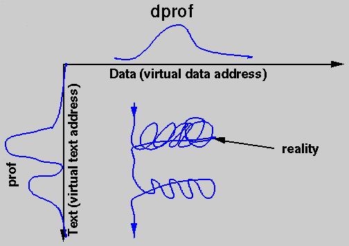
Speedshop and perfex profile the execution path, but there is a second dimension to program behavior: data references.
The dprof tool, like ssrun, executes a program and samples the program while it runs. Unlike ssrun, dprof does not sample the PC and stack. It samples the current operand address of the interrupted instruction, and accumulates a histogram of access to data addresses, grouped in virtual page units. The following is an example of running dprof on adi2:
% dprof -hwpc -out adi2.dprof adi2
 Time:     27.289 seconds
 Checksum:  5.6160428338E+06
% ls -l adi2.dprof
-rw-r--r--    1 guest      40118 Dec 18 18:54 adi2.dprof
% cat adi2.dprof
--------------------------------------------------
   address     thread       reads          writes
--------------------------------------------------
0xfffeff4000     0            168              11
0xfffeff8000     0            228               7
0xfffeffc000     0            156              11
0xffff000000     0            126               7
0xffff004000     0            153               9
0xffff008000     0             71              12
0xffff00c000     0             40               3
0xffff010000     0            116              10
0xffff014000     0            219              38
0xffff018000     0            225              73
0xffff01c000     0            193              53
0xffff020000     0            127              41
0xffff024000     0            246              31
0xffff028000     0            147              18
0xffff02c000     0             50              23
0xffff030000     0             87              47
0xffff034000     0            134              36
0xffff038000     0            165              37
0xffff03c000     0            136              37
0xffff040000     0             98              32
...
0xfffffe8000     0            389              46
0xfffffec000     0            481              50
0xffffff0000     0            262              36
0xffffff4000     0             35               8
Each line contains a count of all references from one program thread (one IRIX process, but this program has only a single process) to one virtual memory page. (The addresses at the left increment by 0x04000, or 16KB.)
dprof operates by statistical sampling; it does not record all references. The time base is either the interval timer (option -itimer) or the R10000 event cycle counter (option -hwpc). The default interrupt frequency using the cycle counter samples only about 1 instruction in 10000. This produces a coarse sample that is not likely to be repeatable from run to run. However, even this sampling rate slows program execution by almost 3 times.
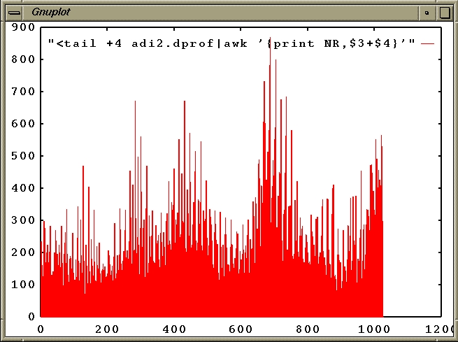
You can obtain a more detailed sample by specifying a shorter overflow count (option -ovfl), but this will extend program execution time proportionately. The coarse histogram is useful for showing which pages are used. For example, you can plot the data as a histogram. Using gnuplot (which is available on the SGI Freeware CDROM), a simple plot of total access density is obtained as follows:
% /usr/freeware/bin/gnuplot

        G N U P L O T
        unix version 3.5
        patchlevel 3.50.1.17, 27 Aug 93
        last modified Fri Aug 27 05:21:33 GMT 1993

        Copyright(C) 1986 - 1993   Thomas Williams, Colin Kelley

        Send comments and requests for help to info-gnuplot@dartmouth.edu
        Send bugs, suggestions and mods to bug-gnuplot@dartmouth.edu

Terminal type set to 'x11'
gnuplot> plot "<tail +4 adi2.dprof|awk '{print NR,$3+$4,$2}'" with box
For this is a single-threaded application, the information provided by dprof is not of great benefit. But for multi-threaded applications, it can reveal quite a lot. Since access to the local memory is faster than access to remote memories on an Origin system, the best performance on parallel programs which sustain a lot of cache misses will be achieved if you can arrange it so that each thread primarily accesses its local memory. dprof gives you the ability to analyze which regions of virtual memory each thread of a program accesses. Since dprof's utility is primarily for multi-threaded applications, we will postpone a more detailed look at how it can be used until later.
Once the amount of code to be tuned has been narrowed down, it's time to actually do the work of tuning. The most important tool available for accomplishing this is the compiler. Ideally, the compiler should be able to automatically make your program run its fastest. But this simply isn't possible because the compiler does not have enough information to always make optimal decisions.
As an example consider a program which obtains its input data from a file. The size of the data are not known until run time. For those data sets which are too big to fit in cache, the best performance will be achieved if the compiler has performed cache optimizations on the code. But for those data sets which do fit in cache, these optimizations should not be done since they will add overhead and make the program run somewhat slower. So what should the compiler do?
Most compilers are limited in the cache optimizations they can perform, so they optimize for in-cache code; this is the case for the MIPSpro 6.x compilers. The nice aspect of this choice is that it makes it fairly easy to verify that the compiler has properly optimized a program: The transformations it makes apply to relatively small sections of code --- typically loops --- and in the case of the MIPSpro 6.x compilers, "report cards" can be generated to show how well each loop has been optimized. Unfortunately, most data sets don't fit in cache, so the loop-by-loop report cards usually don't indicate the true performance of the program.
The MIPSpro 7.x compilers, however, can perform extensive cache optimizations. If you request the highest optimization level, the compiler will optimize for data which do not fit in cache. This means that the majority of programs will benefit from the cache optimizations. But those programs which operate on in-cache data, or in which the programmer has manually made cache optimzations, may have to pay a performance penalty. Fortunately, this penalty will typically be small compared to the advantage most programs gain from cache optimzations. So, given that the compiler must make a choice, this is on balance the right one. However, it does mean that if you understand what your program is doing, you may be able improve its performance by selectively enabling and disabling the compiler's cache optimizations.
This, of course, applies to the other optimizations as well, and is the subject of the following sections. Coming up, we will look at the types of optimizations the compiler is capable of performing and the switches which enable or disable them. For ease of exposition, we will describe the various optimizations in separate sections as if they are independent of each other. The major categories of optimizations covered will include
In reality, these optimizations are not independent of each other: some loop nest optimizations can enhance software pipelining, and inter-procedural analysis can give the loop nest optimizer more information from which to better do its job. As a result, there is perhaps no best order in which to describe them. The above order is convenient, however, since it starts with operations which are fairly localized (i.e., loops) and then progresses to more complicated and global transformations (i.e., cache optimizations).
This order, however, should not be construed as a ranking of their importance in helping your program achieve its best performance. To the contrary, the loop nest optimzations are probably the most important in this respect since they attempt to make your program more cache-friendly. Since these optimizations can be complicated and understanding them requires a knowledge of how caches work, many users will prefer to just let the compiler accomplish what it can automatically. However, for sophistocated users who wish greater control over cache optimizations, the compiler does allow great flexibility in how they are applied. This topic is significant enough that the loop nest optimizations, along with the principles of cache optimizations, will be discussed in a separate section following the other compiler optimzations.
Given that the various optimizations the compiler will perform can interact with each other, it is impossible to provide a simple formula specifying which optimizations should be attempted in which order to achieve the best results in all cases. Nevertheless, we can make some recommendations which work well in general. A good set of compiler flags to use are the following:
-n32 -mips4 -Ofast=ip27 -OPT:IEEE_arithmetic=3
These flags:
In addition, when linking in math routines, be sure to use the fast math library:
-lfastm -lm
These flags can be used to compile and link in one step:
% cc -n32 -mips4 -Ofast=ip27 -OPT:IEEE_arithmetic=3 \
        -o program program.c -lfastm -lm
or separately:
% cc -n32 -mips4 -Ofast=ip27 -OPT:IEEE_arithmetic=3 -c program.c
% cc -n32 -mips4 -Ofast=ip27 -OPT:IEEE_arithmetic=3 \
        -o program program.o -lfastm -lm
Using this set of flags will get you a good deal of the way towards optimal performance. For some users, this will be more than adequate, so we will finish this section by first showing you how you can easily get into the habit of using these recommended flags, and after that we will describe them in a little more detail. In the following sections, we'll present material for users who want to know more than just the basic optimization flags.
In order to make using these flags convenient, it is recommended to get
in the habit of defining makefile variables for them. Below is an example
of a good starting point for a Makefile; for a simply-constructed program, this may be all you need:
#! /usr/sbin/smake
#
FC      = $(TOOLROOT)/usr/bin/f77
CC      = $(TOOLROOT)/usr/bin/cc
LD      = $(FC)
F77     = $(FC)
SWP     = swplist
RM      = /bin/rm -f
MP      =
ABI     = -n32
ISA     = -mips4
PROC    = ip27
ARCH    = $(MP) $(ABI) $(ISA)
OLEVEL  = -Ofast=$(PROC)
FOPTS   = -OPT:IEEE_arithmetic=3
COPTS   = -OPT:IEEE_arithmetic=3
FFLAGS  = $(ARCH) $(OLEVEL) $(FOPTS)
CFLAGS  = $(ARCH) $(OLEVEL) $(COPTS)
LIBS    = -lfastm
LDFLAGS = $(ARCH) $(OLEVEL)
PROF    =

FOBJS   = f1.o f2.o f3.o
COBJS   = c1.o c2.o c3.o
OBJS    = $(FOBJS) $(COBJS)
EXEC    = executable

$(EXEC):        $(OBJS)
        $(LD) -o $@ $(PROF) $(LDFLAGS) $(QV_LOPT) $(OBJS) $(LIBS)

clean:
        $(RM) $(EXEC) $(OBJS)

.SUFFIXES:
.SUFFIXES: .o .F .c .f .swp

.F.o:
        $(FC)  -c $(FFLAGS) $(QV_OPT) $(DEFINES) $<

.f.o:
        $(FC)  -c $(FFLAGS) $(QV_OPT) $(DEFINES) $<

.c.o:
        $(CC)  -c $(CFLAGS) $(QV_OPT) $(DEFINES) $<

.F.swp:
        $(SWP) -c $(FFLAGS) $(QV_OPT) $(DEFINES) -WK,-cmp=$*.m $<

.f.swp:
        $(SWP) -c $(FFLAGS) $(QV_OPT) $(DEFINES) -WK,-cmp=$*.m $<

.c.swp:
        $(SWP) -c $(CFLAGS) $(QV_OPT) $(DEFINES) $<
Such a Makefile can even be generated automatically with a simple script, which we call makemake. To use it, create a directory for your program and move the source files
into the directory. Then, if makemake is in your path, you can create a Makefile for the program by simply typing
% makemake executable
where executable is the name you choose for the program. The script will automatically identify
all the C and Fortran files in the directory and list them in the Makefile for you. To build the program, type
% make
and the recommended flags will automatically be used. A version suitable for debugging can be built with the following command:
% make OLEVEL=-g
To add extra compilation options, use the DEFINES variable. For example:
% make DEFINES="-DDEBUG -OPT:alias=restrict"
To remove the executable and objects:
% make clean
The basic optimization flag is -On, where n is 0, 1, 2, 3, or fast. This flag controls which optimizations the compiler will attempt; the higher the optimization level, the more aggressive the optimizations that will be tried. This has an impact on compilation time: in general, the higher the optimization level, the longer the module will take to compile.
Program modules which consume a noticeable fraction of run time should be compiled with the highest level of optimization. This may be specified with either -O3 or -Ofast. Both flags enable software pipelining and loop nest optimizations. The difference between the two is that -Ofast includes additional optimizations such as inter-procedural analysis (-IPA), arithmetic rearrangements which might cause numerical roundoff differences (-OPT:roundoff=3), and interprets ceratin pointer variables as being independent of one another, which allows faster code to be generated (-OPT:alias=typed). In addition, -Ofast takes an optional argument to allow it to specify to which machine it should target the generated code. For an Origin2000, one should use -Ofast=ip27.
For modules which consume a smaller fraction of the program's runtime, the optimization level used is determined by how much time one is willing to allow for compilation. If compilation time is not an issue, it is easiest to use -O3 or -Ofast=ip27 for all modules. If it is desireable to reduce compilation time, a lower optimzation level may be used for non-performance-critical modules. -O2, or equivalently -O, performs extensive optimzations, but they are generally conservative. That is, they almost always improve runtime performance, and they won't cause numerical roundoff differences; sophistocated optimizations, such as software pipelining and loop nest optimzations, are not performed. -O2 takes longer to compile than -O1, so the latter may be used when there is a strong need to reduce compile time. At this level only very simple optimizations are performed.
The lowest optimzation level, -O0, should only be used when debugging your program. The purpose of this flag is to turn off all optimizations so that there is a direct correspondence between the original source code and the machine instructions the compiler generates; this allows a source-level debugger to show you exactly where in your program the currently executing instruction is. If you don't specify an optimization level, this is what you get, so be sure to explicitly specify the optimization level you want.
-r10000, -TARG:proc=r10000 & -TARG:platform=ipxxWhile the R10000, R8000 and R5000 all support the MIPS IV instruction set architecture, their hardware implementations are quite
different. Code scheduled for one chip will not necessarily run optimally
on another. One can instruct the compiler to generate code optimized for
a particular chip via the -r10000, -r8000 and -r5000 flags. When used while linking, these flags will cause libraries optimized
for the specified chip, if available, to be linked in rather than generic
versions; specially optimized versions of libfastm exist for both the R8000 and R10000. An alternative flag, -TARG:proc=(r4000|r5000|r8000|r10000), will generate code optimized for the specified chip without affecting
which libraries are linked in. If -r10000 has been used, -TARG:proc=r10000 is unnecessary.
In addition to specifying the target chip, one can also specify the target processor board. This gives the compiler information about various hardware parameters, such as cache sizes, which can be used in some optimzations. One can specify the target platform with the -TARG:platform=ipxx flag. For Origin2000, -TARG:platform=ip27 should be used.
Note that if the -Ofast=ip27 flag has been used, one does not need to to use the -r10000, -TARG:proc=r10000 or -TARG:platform=ip27 flags.
-OPT:IEEE_arithmeticThis option controls how strictly the compiler should adhere to the IEEE 754 standard. There is flexibility here for a couple of reasons:
do i = 1, nb(i) = a(i)/cenddo
to
      tmp = 1.0/c
      do i = 1, n
         b(i) = a(i)*tmp
      enddo
is not allowed by the IEEE standard since multiplying by the reciprocal (even a completely IEEE accurate representation of it) rather than dividing can produce results that differ in the least significant place.
For most programs, such strict adherence to the standard is not necessary. This flag provides a way for the user to inform the compiler to what degree it may relax strict IEEE compliance.
This flag permits three levels of conformance as described by the f77(1) man page:
-OPT:IEEE_arithmetic=n
    Specify the level of conformance to IEEE 754 floating point
    arithmetic roundoff and overflow behavior. At level 1 (the
    default), do no optimizations which produce less accurate
    results than required by IEEE 754. At level 2, allow the use
    of operations which may produce less accurate inexact results
    (but accurate exact results) on the target hardware.
    Examples are the recip and rsqrt operators for a MIPS IV
    target. At level 3, allow arbitrary mathematically valid
    transformations, even if they may produce inaccurate results
    for IEEE 754 specified operations, or may overflow or
    underflow for a valid operand range. An example is the
    conversion of x/y to x*recip(y) for MIPS IV targets. See
    also roundoff below.
In general, we recommend using the -OPT:IEEE_arithmetic=3 flag.
-OPT:roundoffThe order in which arithmetic operations are coded into a program dictates the order in which they are to be carried out. For example, the Fortran statement
a = b + c + d + e
specifies that b shall first be added to c, then the result added to d, then the result of that added to e, and finally the result of this last addition shall be stored in a. Most of the time, adhering to such a strict order is more than is required
to produce numerically valid results. In addition, it is likely to restrict
the compiler from taking advantage of all the hardware resources available
(i.e., pipelined floating point units).
The -OPT:roundoff flag allows the user to specify how strictly the compiler must adhere to
such coding order semantics. Like the -OPT:IEEE_arithmetic flag above, there are several levels. The lowest level enforces strict
compliance, while higher levels permit the compiler more freedom to efficiently
use the available hardware at the expense of generating results with numerical
roundoff different than that generated by the strict order. The four levels
are described in the f77(1) man page as follows:
-OPT:roundoff=n
    Specify the level of acceptable departure from source
    language floating-point round-off and overflow semantics.  At
    level 0 (the default at optimization levels -O0 to -O2), do
    no optimizations which might affect the floating-point
    behavior.  At level 1, allow simple transformations which
    might cause limited round-off or overflow differences
    (compounding such transformations could have more extensive
    effects).  At level 2 (the default at optimization level -
    O3), allow more extensive transformations, such as the
    execution of reduction loop iterations in a different order.
    At level 3, any mathematically valid transformation is
    enabled.  Best performance in conjunction with software
    pipelining normally requires level 2 or above, since
    reassociation is required for many transformations to break
    recurrences in loops.  See also IEEE_arithmetic
    above.
In general, we recommend using the -OPT:roundoff=3 flag, but use of this flag is not always without consequences. The reassociations
permitted by this flag will cause the roundoff characteristics of the program
to change. Generally this is not a problem, but in some instances the program's
results can be different enough from what had previously been obtained so
as to be considered wrong. While such a situation may call into question
the numerical stability of the program, the easiest course of action may
be to drop the -OPT:roundoff=3 flag in order to generate the expected results.
The -Ofast flag enables -OPT:roundoff=3. If you are using -Ofast and wish to turn down the roundoff level, you will need to explicitly set
the desired level:
% cc -n32 -mips4 -Ofast=ip27 -OPT:roundoff=2 ...
Using -Ofast implies the use of one additional flag, namely -OPT:alias=typed. This flag specifies the aliasing model to be typed. The aliasing model tells the compiler how to treat potential dependencies caused by dereferencing pointer variables. Without information from the user, the compiler needs to be cautious and assume any two pointers can point to the same location in memory. This caution removes many optimization opportunities, particularly for loops.
To fully understand the implications of this, we'll first need to see how the compiler optimizes loops. This is done via software pipelining, which is covered next. After that, we'll finish the discussion of aliasing models.
Loops contain parallelism. This ranges from, at minimum, instruction-level parallelism, up to parallelism sufficient to carry out different iterations of the loop on different processors. We will deal with multi-processor parallelism later; now we want to concentrate on instruction-level parallelism.
Consider the following loop which implements the vector operation DAXPY:
do i = 1, ny(i) = y(i) + a*x(i)enddo
This adds a vector multiplied by a scalar to a second vector, overwriting the second vector. Each iteration of the loop requires the following instructions:
The R10000 employs a superscalar architecture capable of executing up to 4 instructions per cycle. These superscalar slots may be filled from the following menu:
In addition, all instructions are pipelined and have associated pipeline latencies ranging from 1 to dozens of cycles. It is up to the compiler to figure out how to best schedule the instructions to fill up as many superscalar slots as possible and run the loop at top speed. Software pipelining is a compiler technique for optimally filling the superscalar slots.
Software pipelining does for loops what hardware pipelining does to speedup hardware instructions. In hardware pipelining, an instruction is decomposed into several atomic operations. Separate hardware is built to execute each atom of work. By overlapping instructions in time, all of the hardware can be run concurrently, each piece operating on an atom from a different instruction. The parallelism is not perfect: there is a pipeline startup phase in which one extra stage of the pipeline may run on each new cycle, and there is a pipeline drain phase, where one unit completes its work on each cycle. But if the number of instructions to carry out is large, these will be swamped by the time spent in the steady-state portion of the pipeline, so the performance will approach that of perfect parallelism.
In sofware pipelining, each loop iteration is broken up into instructions as was done above for DAXPY. The iterations are then overlapped in time in an attempt to keep all the functional units busy. Of course, not every loop can keep all the functional units busy; for example, a loop that does no floating point will not use the floating point adder or multiplier. And some units will be forced to remain idle on some cycles in order to observe the pipeline latencies or since only four instructions can be selected from the above menu. Nevertheless, the compiler can determine the minimum number of cycles required for the steady-state portion of the pipeline, and it will try to schedule the instructions so that this level of performance is approached as the number of iterations in a loop increases.
Do note, however, that in calculating the minimum number of cycles required for the loop, the compiler assumes the data are in-cache (more specifically, in the primary data cache). If the data are not in-cache, the loop will take longer to execute. In this case, the code can generally be made to run faster if the compiler generates some additional instructions to prefetch the data from memory into the cache well before they are needed. This is one of the cache optimizations we will describe later. But for the remainder of this discussion of software pipelining, we will only consider in-cache data. This makes it much easier to determine if the software pipeline steady-state has achieved the peak rate the loop is capable of. In the examples which follow, however, this will require disabling the cache optimizations since they are performed automatically when the recommended flags are used. We hope this does not cause any confusion.
To see how effective software pipelining is, we return to the DAXPY example and consider its instruction schedule. We'll state in advance, though, that optimal performance for this loop is 1/3 of the peak floating point rate of the processor since three memory operations are done for each multiply-add, and the processor is capable of at most one memory instruction and one multiply-add per cycle.
Below is the simplest schedule one could come up with for an iteration of this loop:
Cycle 0: ld x x++
Cycle 1: ld y
Cycle 2:
Cycle 3: madd
Cycle 4:
Cycle 5:
Cycle 6: st y br y++
In creating a schedule, several hardware restrictions must be observed:
The simple schedule for this loop achieves 2 floating point operations in 7 cycles, or 1/7 of peak (while a madd is a single instruction, it performs two floating point operations).
We can improve over this schedule by unrolling the loop so that it caclulates 2 vector elements per iteration:
do i = 1, n-1, 2
y(i+0) = y(i+0) + a*x(i+0)
y(i+1) = y(i+1) + a*x(i+1)
enddo
do i = i, n
y(i+0) = y(i+0) + a*x(i+0)
enddo
The schedule for the steady-state part of the unrolled loop is
Cycle 0: ld x0
Cycle 1: ld x1
Cycle 2: ld y0 x+=4
Cycle 3: ld y1 madd0
Cycle 4: madd1
Cycle 5:
Cycle 6: st y0
Cycle 7: st y1 y+=4 br
This loop achieves 4 floating point operations in 8 cycles, or 1/4 of peak; it's closer to the top rate of 1/3 of peak, but still not perfect.
Here is a compiler-generated software pipelined schedule:
[ windup code ]
loop:
Cycle 0: ld y4
Cycle 1: st y0
Cycle 2: st y1
Cycle 3: st y2
Cycle 4: st y3
Cycle 5: ld x5
Cycle 6: ld y5
Cycle 7: ld x6
Cycle 8: ld x7 madd4
Cycle 9: ld y6 madd5
Cycle 10: ld y7 y+=4 madd6
Cycle 11: ld x0 bne out madd7
Cycle 0: ld y0
Cycle 1: st y4
Cycle 2: st y5
Cycle 3: st y6
Cycle 4: st y7
Cycle 5: ld x1
Cycle 6: ld y1
Cycle 7: ld x2
Cycle 8: ld x3 madd0
Cycle 9: ld y2 madd1
Cycle 10: ld y3 y+=4 madd2
Cycle 11: ld x4 beq loop madd3
out:
[ winddown code ]
This loop achieves 8 floating point operations in 12 cycles, or 1/3 of peak, so its performance is optimal. Let's investigate how it works.
The software pipelined schedule consists of 2 blocks of 12 cycles. Each block is called a replication since the same code pattern repeats for each 12-cycle block. There are four madds and twelve memory operations per repliction (as well as a pointer increment and a branch), so each replication achieves the peak calculation rate. Iterations of the loop are spread out over the replications in a pipeline so that the superscalar slots are filled up.
The diagram below shows the memory operations and madds for twelve iterations of the DAXPY loop. Time, in cycles, runs horizontally across the diagram. During the first five iterations, the software pipeline is filled. This is the windup stage; for ease of presentation, it was omitted from the schedule above. Cycles 9 through 20 make up the first replication; cycles 21 through 32 the second replication; and so on. The compiler has unrolled the loop four times, so each replication completes four iterations. Each iteration is spread out over several cycles: 15 for the first of the four unrolled iterations, 10 for the second, and 9 for each of the third and fourth iterations. Since only one memory operation may be executed per cycle, these four iterations must be offset from each other, and it takes 18 cycles to complete all four of them. Two replications are required to contain the full 18 cycles of work for the four iterations. This is more than the minimum latency required to calculate four iterations (we saw above that this could be done in 14 cycles), but spreading the work out allows the iterations to be interleaved into a perfect pipeline.
A test is done at the end of each iteration to determine if all groups of four iterations have been started. If not, execution drops through to the next replication or branches back to the first replication at the beginning of the loop. If all groups of four iterations have begun, execution jumps out to code which will finish the in-progress iterations. This is the winddown code; for ease of presentation, it was omitted from the schedule above.
Due to the 18-cycle latency, a group of four iterations will begin in one replication, continue through the next, and wrap back around to the replication it started in. In the schedule above, numbers only appear for 8 iterations since this is sufficient to account for all operations in two replications. Higher numbered iterations are mapped to one of these 8 iterations using mod 8 arithmetic.
In order to help the user determine how effective the compiler has been at software pipelining, the compiler can generate a report card for each loop. The user can request that these report cards be written to a listing file, or assembler output can be generated to see them.
As an example, once again consider the DAXPY loop:
subroutine daxpy(n,a,x,y)
integer n
real*8 a, x(n), y(n)
c
      do i = 1, n
         y(i) = y(i) + a*x(i)
      enddo
c
return
end
The software pipelining report card can be generated in two ways:
-S flag to generate an assembler file; the report card will be mixed in with
the assembly code. (The flag -LNO:opt=0 is used to prevent certain cache optimzations from being performed which would obscure our current study of software
pipelining; this flag will be described later.)
% f77 -n32 -mips4 -Ofast -OPT:IEEE_arithmetic=3 -LNO:opt=0 \
        -S daxpy.f
awk script swplist which generates the assember file, extracts the report cards, and inserts
each into a source listing file just above the loop it pertains to; the
listing file is given the same name as the file compiled, but with the extension .swp. swplist is used with the same options one uses to compile:
% swplist -n32 -mips4 -Ofast -OPT:IEEE_arithmetic=3 -LNO:opt=0 \
        -c daxpy.f
The report card generated by either of these methods is
 #<swps>
 #<swps> Pipelined loop line 6 steady state
 #<swps>
 #<swps>    50 estimated iterations before pipelining
 #<swps>     2 unrollings before pipelining
 #<swps>     6 cycles per 2 iterations
 #<swps>     4 flops        ( 33% of peak) (madds count as 2)
 #<swps>     2 flops        ( 16% of peak) (madds count as 1)
 #<swps>     2 madds        ( 33% of peak)
 #<swps>     6 mem refs     (100% of peak)
 #<swps>     3 integer ops  ( 25% of peak)
 #<swps>    11 instructions ( 45% of peak)
 #<swps>     2 short trip threshold
 #<swps>     7 ireg registers used.
 #<swps>     6 fgr registers used.
 #<swps>
The purpose of the report card is to give us information as to how effectively the processor's hardware resources are being used in the schedule generated for the loop. There are lines showing how many instructions of each type there are per replication, and what percentage of each resource's peak utilization has been achieved. Let's look in detail at this information.
The report card is for the loop occurring at line 5 of the source file (the compiler reports a line number that is off by 1 in this case). The loop was unrolled 2 times and then software pipelined. The schedule generated by the compiler requires 6 cycles per replication, and each replication retires 2 iterations due to the unrolling.
The steady-state performance of the loop is 33% of the floating point peak. The "madds count as 2" line counts floating point operations. This indicates how fast the processor can run this loop on an absolute scale. Since the peak rate of the processor is 390 MFLOPS (2 floating point operations per cycle with a clock rate of 195 MHz), the steady-state portion of the loop runs at 130 MFLOPS.
Alternatively, the "madds count as 1" line counts floating point instructions. Since the floating point work in most loops does not consist entirely of madd instructions, this count indicates how much of the floating point capablities of the chip are being utilized in the loop given its particular mix of floating point instructions. A 100% utilization here, even if the floating point operation rate is less than 100% of peak, means that the chip is running as fast as it can.
For the R10000, which has an adder and a multiplier, this line does not provide much additional information beyond the "madds count as 2" line. In fact, the utilization percentage is even misleading in this case since all 2 of the floating point instructions in the replication are madds (cf. the next line in the report card), and they use both the adder and multiplier. Here, the instruction is counted as if it simply uses one of the units. On an R8000, for which there are two complete floating point units, each capable of add, multiply and madd instructions, such anomolies do not occur, and this line can provide more information. One can easily see cases in which the chip's floating point units are 100% utilized even though it is not sustaining two floating point operations per unit per cycle.
Each software pipeline replication contains 6 memory references, and this represents 100% utilization of this resource. Thus, this loop is load/store-bound. Sometimes that's the way it is, and no additional (non-memory) resources can make the loop run faster. But in other situations, loops can be re-written to reduce the number of memory operations, and in these cases performance can be improved. We'll see an example of this later.
Only three integer operations are used: a branch and two pointer increments. The total number of instructions for the replication is 11, so there are plenty of free superscalar slots.
The report card indicates that there is a "short trip threshold" of two. This means that for loops with fewer than two (groups of two) iterations, a separate, non-software-pipelined piece of code will be used. Since building up and draining the pipeline imposes some overhead, pipelining is avoided for very short loops.
Finally, we see that 7 integer registers (ireg) and 6 floating point registers (fgr) were required by the compiler to schedule the code. Although not an issue in this case, bigger and more complicated loops will require more registers, sometimes more than physically exist. In these cases, the compiler must either introduce some scratch memory locations to hold intermediate results, thus increasing the number of load and store operations for the loop, or stretch out the loop to allow greater reuse of the existing registers. Should these problems occur, splitting the loop into smaller pieces can often eliminate them.
This report card provides valuable information to the user. If a loop is running well, that will be validated by the information it contains. If the speed of the loop is disappointing, it will provide clues as to what should be done --- either via the use of additional compiler flags or by modifying the code --- to improve the performance.
The compiler will not software pipeline loops by default. In order to enable
software pipelining, the highest level of optimization, -O3, must be used. This can be specified with either -Ofast, as above, or simply with -O3; the difference is that -Ofast is a superset of -O3, and also turns on other optimizations such as inter-procedural analysis. (Alternatively, the switch -SWP:=ON can be used with lower levels of optimization, but -O3 also enables loop nest and other optimizations which are desireable in conjunction with software
pipelining, so this alternative is not recommended.)
The reason that software pipelining is not done by default is that it increases compilation time. While finding the number of cycles in an optimal schedule is easy, producing a schedule given a finite number of registers is a difficult task. Heuristic algorithms are employed to try to find a schedule. In some instances they will fail, and only a schedule with more cycles than optimal can be generated. The schedule which is found can vary depending on subtle code differences or the choice of compiler flags.
Some loops are well-suited to software pipelining. In general, vectorizable loops, such as the DAXPY example above, will software pipeline well with no special effort from the user. But getting some loops to software pipeline can be difficult. Coming up, we'll see that software pipelining cannot be done on loops containing function calls, and it can be impeded when loops are very large or contain recurrences. Fortunately, inter-procedural analysis, loop nest optimizations, and the use of compiler directives can often help in these situations.
For an in-order superscalar processor such as the R8000, it is essential that the key loops in a program be software pipelined in order to achieve good performance; the functional units will sit idle if concurrent work is not scheduled for them. With its out-of-order execution, the R10000 can be much more forgiving of the code generated by the compiler; even code scheduled for another processor can still run well. Nevertheless, there is a limit to the instruction reordering the processor can accomplish, so getting the most time consuming loops in a program to software pipeline is still key to achieving top performance.
Not all loops will software pipeline. One of the most common causes for this is a subroutine or function call inside the loop. When a loop contains a call, the software pipelining report card is:
 #<swpf> Loop line 6 wasn't pipelined because:
 #<swpf>       Function call in the DoBody
 #<swpf>
If the subroutine contains loops of its own, then this software pipelining failure is generally inconsequential since it is the loops inside the subroutine that will need to be software pipelined. However, if there are no loops in the subroutine, finding a way to get the loop containing it to software pipeline may be important for achieving good performance.
Failures of this sort can be remedied by inlining the subroutine or functiion which appears in the loop. This could be done manually, but the compiler can often do this automatically via the inlining features of inter-procedural analysis. Inlining will be discussed later.
In addition, while-loops and loops which contain goto statements which jump out of the loop will not software pipeline. Due to the out-of-order execution ability of the R10000, such non-software pipelined loops can still run with acceptable speeds on Origin2000 systems. However, for in-order processors such as the R8000, such loops could incur a significant performance penalty, so if an alternate implementation which converts the loop to a standard do- or for-loop exists, it should be used.
The -Ofast (or at least -O3) flag is the single most important compiler option to know about and use
since it enables software pipelining, inter-procedural analysis (with -Ofast), loop nest and many other optimizations. But there are a handful of other options
and directives which can also very useful since they can improve the software
pipelined schedules the compiler generates and speed up non-software pipelined
code as well. We will describe those next before delving into fine tuning
inter-procedural analysis and loop nest optimizations.
-OPT:alias=restrict and -OPT:alias=disjointIn order to optimize code effectively, the compiler needs to analyze the
data dependencies in the program. For standard Fortran, this task is made
easier since the language specifies that non-equivalenced arrays of different names do not alias each other, that is, the pieces
of memory they represent do not overlap. When pointers are used --- and
hence this is particularly applicable to C programs --- determining aliasing
information can be impossible. Thus, in any ambiguous situation, the compiler
needs to play it safe and assume aliasing is possible. Unfortunately, this
can severly limit the types of optimizations the compiler can do, and it
can cause many important loops to fail to software pipeline.
A programmer, however, often knows much more about the actual aliasing behavior
than is apparant in the program. The -OPT:alias flag may be used to convey this extra information to the compiler. There
are several different aliasing models which may be used, as described in
the cc(1) man page:
-OPT:alias=name
    Specify the pointer aliasing model to be used.  If name is
    any, then the compiler will assume that any two memory
    references may be aliased unless it can determine otherwise
    (the default).  If name is typed, the ANSI rules for object
    reference types (Section 3.3) are assumed - essentially,
    pointers of distinct base types are assumed to point to
    distinct, non-overlapping objects. If name is no_typed,
    pointers to different base types may point to the same
    object.  If name is unnamed, pointers are also assumed never
    to point to named objects. If name is no_unnamed, pointer
    may point to named object.  If name is no_restrict, distinct
    pointer variables may point to overlapping storage.  If name
    is restrict, distinct pointer variables are assumed to point
    to distinct, non-overlapping objects.  If name is
    no_disjoint, distinct pointer expressions may point to
    overlapping storage.  If name is disjoint, distinct pointer
    expressions are assumed to point to distinct, non-
    overlapping objects.  The restrict and disjoint options are
    unsafe, and may cause existing C programs to fail in obscure
    ways, so it should be used with extreme care.
If it is the case that different pointers point to non-overlapping regions
of memory, then the -OPT:alias=restrict flag should be used to allow the compiler to generate the best performing
code. Note, though, that if this flag is used in a situation in which pointers
can alias the same data, incorrect code can be generated. This is not a compiler problem: it is a case of the user providing the
compiler with false information.
As an example, consider the following C implementation of DAXPY:
void
daxpy(int n, double a, double *x, double *y)

{
  int   i;

  for (i=0; i<n; i++) {
    y[i] += a * x[i];
  }
}
When compiled with
% cc -n32 -mips4 -Ofast=ip27 -OPT:IEEE_arithmetic=3 -LNO:opt=0 \
        -c daxpy.c
the software pipelining message is
 #<swps>
 #<swps> Pipelined loop line 8 steady state
 #<swps>
 #<swps>   100 estimated iterations before pipelining
 #<swps>       Not unrolled before pipelining
 #<swps>     7 cycles per iteration
 #<swps>     2 flops        ( 14% of peak) (madds count as 2)
 #<swps>     1 flop         (  7% of peak) (madds count as 1)
 #<swps>     1 madd         ( 14% of peak)
 #<swps>     3 mem refs     ( 42% of peak)
 #<swps>     3 integer ops  ( 21% of peak)
 #<swps>     7 instructions ( 25% of peak)
 #<swps>     1 short trip threshold
 #<swps>     4 ireg registers used.
 #<swps>     3 fgr registers used.
 #<swps>
 #<swps>     3 min cycles required for resources
 #<swps>     6 cycles required for recurrence(s)
 #<swps>     3 operations in largest recurrence
 #<swps>     7 cycles in minimum schedule found
 #<swps>
(The flag -LNO:opt=0 is used to prevent certain cache optimzations from being performed which would obscure our current study of software pipelining; this flag will be described later.)
Since the compiler cannot determine the data dependencies between x and y, it plays it safe and produces a schedule which is more than twice as slow
as ideal.
Now consider what happens when -OPT:alias=restrict is used:
 #<swps>
 #<swps> Pipelined loop line 8 steady state
 #<swps>
 #<swps>    50 estimated iterations before pipelining
 #<swps>     2 unrollings before pipelining
 #<swps>     6 cycles per 2 iterations
 #<swps>     4 flops        ( 33% of peak) (madds count as 2)
 #<swps>     2 flops        ( 16% of peak) (madds count as 1)
 #<swps>     2 madds        ( 33% of peak)
 #<swps>     6 mem refs     (100% of peak)
 #<swps>     3 integer ops  ( 25% of peak)
 #<swps>    11 instructions ( 45% of peak)
 #<swps>     2 short trip threshold
 #<swps>     7 ireg registers used.
 #<swps>     6 fgr registers used.
 #<swps>
This flag has informed the compiler that the x and y arrays are non-overlapping, so it can generate an ideal schedule. As long
as this subroutine has been specified so that this assumption is correct,
the code will be valid, and it will run significantly faster.
If the code uses pointers to pointers, -OPT:alias=restrict is not sufficient to tell the compiler that data dependencies do not exist.
If this is the case, then -OPT:alias=disjoint should be used to allow the compiler to ignore potential data dependencies.
(Note that -OPT:alias=disjoint is a superset of -OPT:alias=restrict.) As with -OPT:alias=restrict, if these pointers really can point to the same memory location, then the
use of this flag can cause incorrect results.
C code using multi-dimensional arrays is a good candidate for the -OPT:alias=disjoint flag. Consider the following nest of loops:
  for ( i=1; i< size_x1-1 ;i++)
    for ( j=1; j< size_x2-1 ;j++)
       for ( k=1; k< size_x3-1 ;k++)
        {
          out3 = weight3*(    field_in[i-1][j-1][k-1]
                            + field_in[i+1][j-1][k-1]
                            + field_in[i-1][j+1][k-1]
                            + field_in[i+1][j+1][k-1]
                            + field_in[i-1][j-1][k+1]
                            + field_in[i+1][j-1][k+1]
                            + field_in[i-1][j+1][k+1]
                            + field_in[i+1][j+1][k+1] );
          out2 = weight2*(    field_in[i  ][j-1][k-1]
                            + field_in[i-1][j  ][k-1]
                            + field_in[i+1][j  ][k-1]
                            + field_in[i  ][j+1][k-1]
                            + field_in[i-1][j-1][k  ]
                            + field_in[i+1][j-1][k  ]
                            + field_in[i-1][j+1][k  ]
                            + field_in[i+1][j+1][k  ]
                            + field_in[i  ][j-1][k+1]
                            + field_in[i-1][j  ][k+1]
                            + field_in[i+1][j  ][k+1]
                            + field_in[i  ][j+1][k+1] );
          out1 = weight1*(    field_in[i  ][j  ][k-1]
                            + field_in[i  ][j  ][k+1]
                            + field_in[i  ][j+1][k  ]
                            + field_in[i+1][j  ][k  ]
                            + field_in[i-1][j  ][k  ]
                            + field_in[i  ][j-1][k  ] );
          out0 = weight0*     field_in[i  ][j  ][k  ];
          field_out[i][j][k] = out0+out1+out2+out3;
        }
Here, the three-dimensional arrays are declared as
  double***  field_out;
  double***  field_in;
Without input from the user, the compiler cannot tell if there are data
dependencies between different elements of one array, let alone both. Due
to the multiple levels of indirection, even -OPT:alias=restrict does not provide sufficient information. As a result, compiling with
% cc -n32 -mips4 -Ofast=ip27 -OPT:IEEE_arithmetic=3:alias=restrict \
        -c stencil.c
produces the following software pipeline report card:
 #<swps>
 #<swps> Pipelined loop line 77 steady state
 #<swps>
 #<swps>   100 estimated iterations before pipelining
 #<swps>       Not unrolled before pipelining
 #<swps>    42 cycles per iteration
 #<swps>    30 flops        ( 35% of peak) (madds count as 2)
 #<swps>    27 flops        ( 32% of peak) (madds count as 1)
 #<swps>     3 madds        (  7% of peak)
 #<swps>    42 mem refs     (100% of peak)
 #<swps>    16 integer ops  ( 19% of peak)
 #<swps>    85 instructions ( 50% of peak)
 #<swps>     1 short trip threshold
 #<swps>    20 ireg registers used.
 #<swps>    12 fgr registers used.
 #<swps>
However, we can instruct the compiler that even multiple indirections are
independent with the -OPT:alias=disjoint flag. Compiling with this aliasing model instead of the restrict model
produces the following results:
 #<swps>
 #<swps> Pipelined loop line 77 steady state
 #<swps>
 #<swps>   100 estimated iterations before pipelining
 #<swps>       Not unrolled before pipelining
 #<swps>    28 cycles per iteration
 #<swps>    30 flops        ( 53% of peak) (madds count as 2)
 #<swps>    27 flops        ( 48% of peak) (madds count as 1)
 #<swps>     3 madds        ( 10% of peak)
 #<swps>    28 mem refs     (100% of peak)
 #<swps>    12 integer ops  ( 21% of peak)
 #<swps>    67 instructions ( 59% of peak)
 #<swps>     2 short trip threshold
 #<swps>    14 ireg registers used.
 #<swps>    15 fgr registers used.
 #<swps>
This is a 50% improvement in performance, and all it took was a flag to tell the compiler that the pointers can't alias each other.
The -OPT:alias=[restrict|disjoint] flag is very important for C programs. When the information it conveys
is true, it should definitely be used to produce better performing object
code. However, there are some situations when even this flag is insufficient
to produce the best performing code. Consider the loop in the following
C function:
void idaxpy(

int     n,
double  a,
double  *x,
double  *y,
int     *index)

{
  int   i;

  for (i=0; i<n; i++) {
    y[index[i]] += a * x[index[i]];
  }
}
This is the DAXPY operation we have seen before, except now the vector elements
are chosen indirectly through an index array. If the vectors x and y are non-overlapping, we should compile the function with -OPT:alias=restrict. Doing so, and using the other recommended flags (plus -LNO:opt=0 to prevent cache optimzations from obscuring some of the details we are interested in here),
% cc -n32 -mips4 -Ofast=ip27 -OPT:IEEE_arithmetic=3:alias=restrict \
        -LNO:opt=0 -c idaxpy.c
we obtain the following less than optimal results:
 #<swps>
 #<swps> Pipelined loop line 13 steady state
 #<swps>
 #<swps>    50 estimated iterations before pipelining
 #<swps>     2 unrollings before pipelining
 #<swps>    10 cycles per 2 iterations
 #<swps>     4 flops        ( 20% of peak) (madds count as 2)
 #<swps>     2 flops        ( 10% of peak) (madds count as 1)
 #<swps>     2 madds        ( 20% of peak)
 #<swps>     8 mem refs     ( 80% of peak)
 #<swps>     8 integer ops  ( 40% of peak)
 #<swps>    18 instructions ( 45% of peak)
 #<swps>     1 short trip threshold
 #<swps>    10 ireg registers used.
 #<swps>     4 fgr registers used.
 #<swps>
 #<swps>     8 min cycles required for resources
 #<swps>    10 cycles in minimum schedule found
 #<swps>
(When run at optimal speed, this loop should be load-store bound. In that case, the memory references should be at 100% of peak.)
The problem is that since the values of the index array are unknown, there
could be data dependencies between loop iterations for the vector y. For example, if index[i] = 1 for all i, all iterations would update the same vector element. Note that this type
of inter-interation dependency could just as easily arise in a Fortran routine:
      do i = 1, n
         y(index(i)) = y(index(i)) + a * x(index(i))
      enddo
If you know that the values of the array index are such that no dependencies will occur, you can inform the compiler of
this via the ivdep compiler directive. For a Fortran program, the directive looks like
 c$dir ivdep
      do i = 1, n
         y(ind(i)) = y(ind(i)) + a * x(ind(i))
      end
In C, the directive is called a pragma, and its use is as follows:
#pragma ivdep
  for (i=0; i<n; i++) {
    y[index[i]] += a * x[index[i]];
  }
When this modified version of the program is compiled as before, the schedule is improved by 25%:
 #<swps>
 #<swps> Pipelined loop line 14 steady state
 #<swps>
 #<swps>    50 estimated iterations before pipelining
 #<swps>     2 unrollings before pipelining
 #<swps>     8 cycles per 2 iterations
 #<swps>     4 flops        ( 25% of peak) (madds count as 2)
 #<swps>     2 flops        ( 12% of peak) (madds count as 1)
 #<swps>     2 madds        ( 25% of peak)
 #<swps>     8 mem refs     (100% of peak)
 #<swps>     8 integer ops  ( 50% of peak)
 #<swps>    18 instructions ( 56% of peak)
 #<swps>     2 short trip threshold
 #<swps>    14 ireg registers used.
 #<swps>     4 fgr registers used.
 #<swps>
What the ivdep pragma has done is give the compiler permission to ignore the dependencies which are possible from one iteration to the next. As long as the dependencies don't actually occur, correct code will be generated. But if an ivdep directive is used when there really are dependencies, the compiler will generated incorrect code. Just as when using the -OPT:alias=[restrict|disjoint] flag, this would be a case of user error.
There are a few subtleties in how the ivdep directive works; we explain these now. First, we note that the directive applies only to inner loops. Second, it applies only to dependencies which are carried by the loop. Consider the following code segment:
Two types of dependencies are possible in this loop. If index(1,i) = index(1,i+k) or index(2,i) = index(2,i+k) for some value of k such that i+k is in the range 1 to n, then we say there is a loop-carried dependency. If index(1,i) = index(2,i) for some value of i, then there is a non-loop-carried dependency. What we saw above in the idaxpy example was a potential loop-carried dependency. The ivdep directive is used to inform the compiler that the dependency is not actually
present since we know that the values of the index array are never equal. But if the compiler detects potential non-loop-carried
dependencies, the ivdep directive will not instruct the compiler to ignore these potential dependencies.
To do this, the behavior of the ivdep directive needs to be modified via the -OPT:liberal_ivdep=TRUE flag. When this flag is used, an ivdep directive means to ignore all dependencies in a loop.
With either variant of ivdep, the compiler will issue a warning if the directive has instructed it to break an obvious dependence. An example of this is the following:
  for (i=0; i<n; i++) {
     a[i] = a[i-1] + 3;
  }
In this loop the dependence is real, so ignoring it will almost certainly mean producing incorrect results. Nevertheless, an ivdep pragma will break the dependence, and the compiler will issue a warning and then schedule the code so that the iterations are carried out independently.
One more variant of ivdep exists and it is enabled with the flag -OPT:cray_ivdep=TRUE. This instructs the compiler to use the semantics that Cray Research specified when it originated this directive for its vectorizing compilers. That is, only "lexically backwards" loop-carried dependencies are broken. The idaxpy examples above is an instance of a lexically backwards dependence. The example below is not:
  for (i=0; i<=n; i++) {
     a[i] = a[i+1] + 3;
  }
Here, the dependence is from the load (a[i+1]) to the store (a[i]), and the load comes lexically before the store. In this case, a Cray semantics ivdep directive would not break the dependence.
As was seen above in the sections on the -OPT:alias=restrict and -OPT:alias=disjoint flags and the ivdep directive, C code presents the compiler with some data dependency challenges. The
extra information these provide allows one to achieve good performance from
C despite the language semantics. But there are a few other things that
can be done to improve the speed of programs written in C.
Global variables can sometimes cause performance problems since it is difficult for the compiler to determine whether they alias other variables. If loops involving global variables do not software pipeline as efficiently as they should, making local copies of the global variables will often cure the problem.
Another problem arises from using dereferenced pointers in loop tests. For example, the loop
  for (i=0; i<(*n); i++) {
    y[i] += a * x[i];
  }
will not software pipeline since the compiler cannot tell whether *n will change during the loop. If it is known that this value is loop-invariant, one can inform the compiler of this by creating a temporary scalar variable to use in the loop test:
  int   m = *n;

  for (i=0; i<m; i++) {
    y[i] += a * x[i];
  }
This loop will now software pipeline (and if -OPT:alias=[restrict|disjoint] is used, it will achieve optimal performance).
The following example shows a different case of loop-invariant pointers leading to aliasing problems:
void
sub1(

double  **dInputToHidden,
double  *HiddenDelta,
double  *Input,
double  **InputToHidden,
double  alpha,
double  eta,
int     NumberofInputs,
int     NumberofHidden)

{
  int   i;
  int   j;

  for (i=0; i<NumberofInputs; i++) {
    for (j=0; j<NumberofHidden; j++) {
      dInputToHidden[i][j] = alpha * dInputToHidden[i][j] +
                             eta * HiddenDelta[j] * Input[i];
      InputToHidden[i][j] += dInputToHidden[i][j];
    }
  }
}
This loop is similar to a DAXPY: it should be memory bound with about a 50% floating point utilization. But compiling with -OPT:alias=disjoint is not quite sufficient to achieve this level of performance:
 #<swps>
 #<swps> Pipelined loop line 19 steady state
 #<swps>
 #<swps>   100 estimated iterations before pipelining
 #<swps>       Not unrolled before pipelining
 #<swps>     7 cycles per iteration
 #<swps>     5 flops        ( 35% of peak) (madds count as 2)
 #<swps>     4 flops        ( 28% of peak) (madds count as 1)
 #<swps>     1 madd         ( 14% of peak)
 #<swps>     7 mem refs     (100% of peak)
 #<swps>     6 integer ops  ( 42% of peak)
 #<swps>    17 instructions ( 60% of peak)
 #<swps>     3 short trip threshold
 #<swps>    16 ireg registers used.
 #<swps>     8 fgr registers used.
 #<swps>
The problem is the pointers indexed by i: they are causing the compiler to see dependencies which aren't there.
This problem can be fixed hoisting the invariants out of the inner loop:
void
sub2(

double  **dInputToHidden,
double  *HiddenDelta,
double  *Input,
double  **InputToHidden,
double  alpha,
double  eta,
int     NumberofInputs,
int     NumberofHidden)

{
  int   i;
  int   j;
  double        *dInputToHiddeni, *InputToHiddeni, Inputi;

  for (i=0; i<NumberofInputs; i++) {

    /* Hoisting loop invariants sometimes helps software pipelining.
     */
    dInputToHiddeni = dInputToHidden[i];
    InputToHiddeni = InputToHidden[i];
    Inputi = Input[i];

    for (j=0; j<NumberofHidden; j++) {
      dInputToHiddeni[j] = alpha * dInputToHiddeni[j] +
                             eta * HiddenDelta[j] * Inputi;
      InputToHiddeni[j] += dInputToHiddeni[j];
    }
  }
}
Written this way, the compiler can see that dInputToHidden[i], InputToHidden[i] and Input[i] will not change during execution of the j-loop, so it can schedule that loop more aggressively. This version, compiled
with
% cc -n32 -mips4 -Ofast=ip27 -OPT:IEEE_arithmetic=3:alias=disjoint \
        -LNO:opt=0 -c cloop.c
produces
 #<swps>
 #<swps> Pipelined loop line 52 steady state
 #<swps>
 #<swps>   100 estimated iterations before pipelining
 #<swps>       Not unrolled before pipelining
 #<swps>     5 cycles per iteration
 #<swps>     5 flops        ( 50% of peak) (madds count as 2)
 #<swps>     4 flops        ( 40% of peak) (madds count as 1)
 #<swps>     1 madd         ( 20% of peak)
 #<swps>     5 mem refs     (100% of peak)
 #<swps>     4 integer ops  ( 40% of peak)
 #<swps>    13 instructions ( 65% of peak)
 #<swps>     3 short trip threshold
 #<swps>     8 ireg registers used.
 #<swps>    10 fgr registers used.
(The flag -LNO:opt=0 is used to prevent certain cache optimzations from being performed which would obscure our current study of software pipelining; this flag will be described later.)
-TENV:X=nWe saw earlier with the ivdep directive that if extra information is conveyed to the compiler, it can generate
faster code. A useful bit of information which the compiler can sometimes
exploit is: which exceptions may be ignored. An exception is an event which
will require intervention by the operating system. Examples are floating
point exceptions such as divide by 0, or a segmentation fault, which is
a memory exception caused by an invalid memory reference. Any program can
choose which exceptions it will pay attention to and which it will ignore.
For example, floating point underflows will generate exceptions, but since
their effect on the numerical results is usually negligible, they are typically
ignored by flushing them to 0 (via hardware). Divide by 0 is generally enabled
since it usually indicates a fatal error in the program.
How the compiler can take advantage of disabled exceptions is best seen through an example. Consider a program which is known to not make invalid memory references. It will run fine whether memory exceptions are enabled or disabled. But if they are disabled and the compiler knows this, it can generate code which may speculatively make references to potentially invalid memory locations, e.g., reading beyond the end of an array. Such code can run faster than non-speculative code on a superscalar architecture if it takes advantage of functional units which would otherwise be idle. In addition, the compiler can often reduce the amount of software pipeline winddown code when it can make such speculative memory operations; this allows more of the loop iterations to be spent in the steady state code, leading to greater performance.
Speculative code generated by the compiler results in instructions moving in front of a branch which previously had been protecting them from causing exceptions. For example, accesses to memory elements beyond the end of an array are normally protected by the test at the end of the loop. Speculative code can be even riskier. For instance, a code sequence such as
if (x .ne. 0.0) b = 1.0/x
might be changed into
      tmp = 1.0/x
      if (x .ne. 0.0) b = tmp
Thus, division by 0 is no longer protected by the branch. Allowing such speculation is the only way to get some loops to software pipeline. On an in-order superscalar processor such as the R8000, speculation is critical to achieving top performance on loops containing branches. To allow this speculation to be done more freely by the compiler, most exceptions are disabled by default on R8000-based machines.
For the R10000, however, speculation is also done in the hardware. Instructions can be executed out of order, and branches are speculatively executed automatically. Any exceptions encountered via hardware speculation which would not normally occur in the program are dismissed without operating system intervention. Thus, most exceptions are enabled by default in R10000-based systems. Due to the hardware speculation in the R10000, software speculation by the compiler is less critical from a performance point of view. Moreover, it can cause problems since exceptions encountered on a code path generated by the compiler will not simply be dismissed. In the best case, the operating system will need to intervene; in the worst case, such operations can lead to NaNs entering the calculation stream or the program aborting.
For these reasons, when generating code for the R10000, the compiler by
default only performs the safest speculative operations. Which operations
it will speculate on are controlled by the -TENV:X=n flag, where n has the following meanings as described by the f77(1) man page:
-TENV:X=0..4
    Specify the level of enabled exceptions that will be assumed
    for purposes of performing speculative code motion (default
    level 1 at -O0..-O2, 2 at -O3).  In general, an instruction
    will not be speculated (i.e. moved above a branch by the
    optimizer) unless any exceptions it might cause are disabled
    by this option.  At level 0, no speculative code motion may
    be performed.  At level 1, safe speculative code motion may
    be performed, with IEEE-754 underflow and inexact exceptions
    disabled.  At level 2, all IEEE-754 exceptions are disabled
    except divide by zero.  At level 3, all IEEE-754 exceptions
    are disabled including divide by zero.  At level 4, memory
    exceptions may be disabled or ignored.

    NOTE: At levels above the default level 1, various hardware
    exceptions which are normally useful for debugging, or which
    are trapped and repaired by the hardware, may be disabled or
    ignored, with the potential of hiding obscure bugs.  The
    program should not explicitly manipulate the IEEE floating-
    point trap-enable flags in the hardware if this option is
    used.
The default is -TENV:X=1 for optimization levels of -O2 or below, and -TENV:X=2 for -O3 or -Ofast. Programs compiled with higher values of n can suffer from excessive numbers of exceptions as a result of the software
speculation. In many instances, the only negative effect this will have
is on performance, where it shows up as unusually high system time. In other
cases, such as when divides by zero are performed, NaNs and Infinities can
propogate through the calculations ruining the results. The solution to
both these problems is to recompile with a lower value of n.
Although higher than default -TENV:X values can provide a modest increase in performance for programs which one has verified do not generate exceptions, we in general recommended using the default values.
Important Note: If you have compiled the program with a higher than default value for
the -TENV:X flag, you should not use libfpe to enable any exceptions which the compiler now assumes are not enabled.
This could very easily result in the program generating mysterious floating
point exceptions. For example, if you compile with -TENV:X=3, the compiler assumes that floating point divide-by-zero exceptions are
turned off. As a result, it may replace an innocent construct such as
if (x .ne. 0.0) b = 1.0/x
with the following speculative code
tmp = 1.0/x
if (x .ne. 0.0) b = tmp
which may divide by zero. If the divide-by-zero exception is disabled, this
speculative code cannot cause problems since if tmp is ever infinity, it is not stored in b. However, if libfpe has been used to enable the divide-by-zero exception, your program will
abort if the calculation of tmp divides by zero, and it could be pretty painful to figure out what happened.
Most compiler optimizations work within a single procedure (function, subroutine, etc.) at a time. This helps keep the problems manageable, and is a key aspect of supporting separate compilation, because it allows the compiler to restrict attention to the current source file.
However, this intra-procedural focus also presents serious restrictions. By avoiding dependence on information from other procedures, an optimizer is forced to make worst-case assumptions about the possible effects of those procedures. For instance, at boundary points, including all procedure calls, it must typically save (and/or restore) the state of all variables to (from) memory.
By contrast, inter-procedural analysis (IPA) algorithms analyze more than a single procedure --- preferably the entire program --- at once. As a result, they perform optimizations across procedure boundaries, and these results are provided to subsequent optimization phases (such as loop nest optimizations or software pipelining) so that their optimizations benefit.
The optimizations performed by the MIPSpro 7.x compilers's IPA facility include:
IPA is easy to use. All you need do is use an optimization level of -O2 or -O3 and add -IPA to both the compile and link steps when building your program:
% cc -IPA ... -c *.c
% cc -IPA -o program *.o
Alternatively, you may use -Ofast for both compile and link steps since this optimization flag enables IPA.
If there are modules which you would prefer to compile using an optimization level of -O1 or -O0, that's fine. They will link into the program with no problems, but no inter-procedural analysis will be performed on them.
IPA works by postponing much of the compilation process until the link step, when all of the program components can be analyzed together. Schematically, this looks like the following:
The compile step does initial processing of the source file, placing an intermediate representation of the procedures it contains into the output .o file instead of normal relocatable code. Such object files are called WHIRL objects to distinguish them from normal relocatable object files. This processing is really two phases: the normal front end language processing (fe), plus an IPA summary phase which collects local information which will be used by IPA later. Since most back end (be) options (i.e., any of the standard optimization flags, -O3, -OPT:IEEE_arithmetic=3, etc.) are transmitted via the IPA summary phase, they must be present on the command line for the compile step.
The link step, although it is still invoked by a single ld(1) command, becomes several steps. First, the linker invokes IPA, which analyzes and transforms all of the input WHIRL objects together, writing modified versions of the objects. Then it invokes the compiler back end on each of the modified objects, producing a normal relocatable object. Finally, it invokes the linker again for a normal linkage step, producing an executable program or DSO.
Unlike other IPA implementations, the MIPSpro compiler does not require that all of the components of a program be subjected to IPA analysis. The ld(1) command which invokes IPA may include object files (.o) and archives (.a) which have been compiled normally without IPA analysis, as well as referencing DSOs which, however they were compiled, cannot contribute detailed information because the DSO may be replaced with a different implementation after the program is built.
The temporary files created during the expanded link step are all created in a temporary subdirectory of the output program's directory; like other temporary files produced by the compilation process, they are normally removed on completion (unless the -keep option is specified).
When using IPA, the proportion of time spent in compiling and linking will
change. You will typically find that the compile step is faster with IPA
than without; this is because the majority of the optimizations have been
postponed until the link step. Conversely, the link step will take longer
than when IPA is not used since it is now responsible for most of the compilation
work. In addition, the total build time is likely to increase for two reasons:
First, although the IPA step may not be very expensive itself, it usually
increases the size of the code by inlining, and therefore expands the time
required by the rest of the compiler. More importantly, since IPA analysis
can propagate information from one module into optimization decisions in
arbitrary other modules, even minor changes to a single component module
will cause most of the program compilation to be redone. As a result, IPA
is best suited for use on programs with a stable source base. (To avoid
using IPA during code development, and hence save some re-compilation time,
in the recommended flags replace -Ofast with -O3 -r10000 -OPT:roundoff=3, and for code with pointers, also add the appropriate aliasing flag: -OPT:alias=[typed|restrict|disjoint].)
One of the key features of IPA is inlining. This is the replacement of a call to a subroutine or function with the code from that routine. This can improve performance in several ways:
But there are some disadvantages to inlining:
Thus, inlining is does not always improve program execution time. A a result, there are flags you can use to control which routines will be inlined.
There are also some restrictions to inlining. The following types of routines cannot be inlined:
IPA supports two types of inlining: manual and automatic. The manual (also
known as standalone) inliner is invoked with the -INLINE option group. It has been provided to support the C++ inline keyword, but can also be used for C and Fortran programs using the command
line option. It only inlines the routines which you specify, and they must
be located in the same source file as the routine into which they are inlined.
The automatic inliner is invoked whenever -IPA (or -Ofast) is used. It uses heuristics to decide which routines will be beneficial
to inline, so you don't need to specify these explicitly. It can inline
routines from any files which have been compiled with -IPA. We'll now look at how both inliners operate.
The manual inliner is controlled with the -INLINE option group. You need to use a combination of options to specify which routines to inline, and there are 4 options for doing so:
As an example, consider the following code:
      subroutine zfftp ( z, n, w, s )
      real*8 z(0:2*n-1), w(2*(n-1)), s(0:2*n-1)
      integer n
c
      integer iw, i, m, l, j, k
      real*8 w1r, w1i, w2r, w2i, w3r, w3i
c
      iw = 1
c
c     First iteration of outermost loop over l&m: n = 4*lm.
c
      i = 0
      m = 1
      l = n/4
      if (l .gt. 1) then
         do j = 0, l-1
            call load4(w(iw),iw,w1r,w1i,w2r,w2i,w3r,w3i)
            call radix4pa(z(2*(j+0*l)),z(2*(j+1*l)),
     &                    z(2*(j+2*l)),z(2*(j+3*l)),
     &                    s(2*(4*j+0)),s(2*(4*j+1)),
     &                    s(2*(4*j+2)),s(2*(4*j+3)),
     &                    w1r,w1i,w2r,w2i,w3r,w3i)
         enddo
         i = i + 1
         m = m * 4
         l = l / 4
      endif
c
c       .
c       .
c       .
c
      return
      end
The loop (do j ...) contains two subroutine calls. These subroutines contain the following
code:
c
      subroutine load4 ( w, iw, w1r, w1i, w2r, w2i, w3r, w3i )
c
      real*8 w(0:5), w1r, w1i, w2r, w2i, w3r, w3i
      integer iw
c
      w1r = w(0)
      w1i = w(1)
      w2r = w(2)
      w2i = w(3)
      w3r = w(4)
      w3i = w(5)
c
      iw = iw + 6
c
      return
      end
c
c------------------------------------------------------------------------------
c
      subroutine radix4pa ( c0, c1, c2, c3, y0, y1, y2, y3,
     &                      w1r, w1i, w2r, w2i, w3r, w3i )
c
      real*8 c0(0:1), c1(0:1), c2(0:1), c3(0:1)
      real*8 y0(0:1), y1(0:1), y2(0:1), y3(0:1)
      real*8 w1r, w1i, w2r, w2i, w3r, w3i
c
      real*8 d0r, d0i, d1r, d1i, d2r, d2i, d3r, d3i
      real*8 t1r, t1i, t2r, t2i, t3r, t3i
c
      d0r = c0(0) + c2(0)
      d0i = c0(1) + c2(1)
      d1r = c0(0) - c2(0)
      d1i = c0(1) - c2(1)
      d2r = c1(0) + c3(0)
      d2i = c1(1) + c3(1)
      d3r = c3(1) - c1(1)
      d3i = c1(0) - c3(0)

      t1r = d1r + d3r
      t1i = d1i + d3i
      t2r = d0r - d2r
      t2i = d0i - d2i
      t3r = d1r - d3r
      t3i = d1i - d3i

      y0(0) = d0r + d2r
      y0(1) = d0i + d2i
      y1(0) = w1r*t1r - w1i*t1i
      y1(1) = w1r*t1i + w1i*t1r
      y2(0) = w2r*t2r - w2i*t2i
      y2(1) = w2r*t2i + w2i*t2r
      y3(0) = w3r*t3r - w3i*t3i
      y3(1) = w3r*t3i + w3i*t3r

      return
      end
Both subroutines are straight-line code; inlining them will reduce function
call overhead; more importantly, inlining will allow the j-loop to software pipeline.
If all the code is contained in the file fft.f, we can inline the calls with the following compilation command:
% f77 -n32 -mips4 -O3 -r10000 -OPT:IEEE_arithmetic=3:roundoff=3 \
        -INLINE:must=load4,radix4pa -flist -c fft.f
(Here, we have used -O3 -r10000 -OPT:roundoff=3 instead of -Ofast since we don't want -IPA to automatically inline the subroutines!) The -flist flag is used so that the compiler will write out a Fortran file showing what transformations the compiler has done. This file is named fft.w2f.f (where w2f stands for WHIRL-to-Fortran). One can confirm that the subroutines were inlined by checking the w2f file. It contains the code
        l = (n / 4)
        IF(l .GT. 1) THEN
          DO j = 0, l + -1, 1
            w1i = w((j * 6) + 2)
            w2r = w((j * 6) + 3)
            w2i = w((j * 6) + 4)
            w3r = w((j * 6) + 5)
            w3i = w((j * 6) + 6)
            d0r = (z((j * 2) + 1) + z((((l * 2) + j) * 2) + 1))
            d0i = (z((j * 2) + 2) + z((((l * 2) + j) * 2) + 2))
            d1r = (z((j * 2) + 1) - z((((l * 2) + j) * 2) + 1))
            d1i = (z((j * 2) + 2) - z((((l * 2) + j) * 2) + 2))
            d2r = (z(((l + j) * 2) + 1) + z((((l * 3) + j) * 2) + 1))
            d2i = (z(((l + j) * 2) + 2) + z((((l * 3) + j) * 2) + 2))
            d3r = (z((((l * 3) + j) * 2) + 2) - z(((l + j) * 2) + 2))
            d3i = (z(((l + j) * 2) + 1) - z((((l * 3) + j) * 2) + 1))
            t1r = (d1r + d3r)
            t1i = (d1i + d3i)
            t2r = (d0r - d2r)
            t2i = (d0i - d2i)
            t3r = (d1r - d3r)
            t3i = (d1i - d3i)
            s((j * 8) + 1) = (d0r + d2r)
            s((j * 8) + 2) = (d0i + d2i)
            s((j * 8) + 3) = ((w((j * 6) + 1) * t1r) -(w1i * t1i))
            s((j * 8) + 4) = ((w((j * 6) + 1) * t1i) +(w1i * t1r))
            s((j * 8) + 5) = ((w2r * t2r) -(w2i * t2i))
            s((j * 8) + 6) = ((w2r * t2i) +(w2i * t2r))
            s((j * 8) + 7) = ((w3r * t3r) -(w3i * t3i))
            s((j * 8) + 8) = ((w3r * t3i) +(w3i * t3r))
          END DO
        ENDIF
        RETURN
which shows that the two calls were inlined into the loop.
There are two other ways to confirm that the routines have been inlined:
-INLINE:list to instruct the compiler to print out the name of each routine as it is
being inlined.
-S turns off IPA).
Now let's look at IPA's automatic inlining. As the name implies, this is automatic. The only constraints are that the compiler will consider inlining to no longer be beneficial if it increases the size of the program by 100% or more, or if it the extra code causes the -Olimit to be exceeded. (This is the maximum size, in basic blocks, of a routine that the compiler will optimize. Generally, one does not worry about this limit since if it is exceeded, the compiler will print a warning mesage instructing you to to recompile using the flag -Olimit=nnnn. It is described in the reference pages for cc(1) and f77(1).)
If one of these limits is exceeded, IPA will restrict the inlining rather than simply not doing any at all. It decides which routines will remain inlined based on their location in the call hierarchy. Routines at the lowest depth in the call graph are inlined first, followed by routines higher up in the hierarchy. This is illustrated below:
Here, the call tree for a small program is shown on the left. At the lowest depth, n=0, leaf routines (i.e., those which do not call any other routines) are inlined; in this case, the routine E is inlined into routines D and C. At the next level up, n=1, D is inlined into B and C is inlined into A. At the n=2 level, which is the top level for this program, B is inlined into A. IPA will stop automatic inlining at the level which causes the program size to double, or for which the -Olimit is exceeded.
You can increase or decrease the amount of automatic inlining via three -IPA options:
IPA's automatic inlining will inline the calls to load4 and radix4pa in the example above. But since most of IPA's actions are not performed
until the link stage, you won't get a w2f file with which to verify this until the link has been completed:
% f77 -n32 -mips4 -Ofast -OPT:IEEE_arithmetic=3 -flist -c fft.f
% f77 -n32 -mips4 -Ofast -OPT:IEEE_arithmetic=3 -flist -o fft fft_main.f fft.o
//usr/lib32/cmplrs/be translates fft.I into fft.w2f.f, based on source fft.I

--- fft_main.I ---
//usr/lib32/cmplrs/be translates fft_main.I into fft_main.w2f.f, based on source fft_main.I
% f77 -n32 -mips4 -Ofast -OPT:IEEE_arithmetic=3 -flist -c fft2.f
% f77 -n32 -mips4 -Ofast -OPT:IEEE_arithmetic=3 -flist -o fft2 fft2.o
//usr/lib32/cmplrs/be translates fft2.I into fft2.w2f.f, based on source fft2.I
Here, fft_main.f is just a simple main routine which calls zfftp once with the fixed value of n=1024 and then prints out some results (so that the compiler doesn't optimize
away the code!) In this case, not only are load4 and radix4p inlined into zfftp, but zfftp is also inlined into the main routine.
If for some reason we wanted to prevent zfftp from being inlined into the main routine, the -IPA:space and -IPA:forcedepth flags won't be able to help us here. All the subroutine calls in this tiny
example are made just once, so the code is not expanded in size by the inlining.
Thus, restricting the space expansion doesn't accomplish what we want. However,
the -INLINE:must and -INLINE:never flags work in conjunction with the automatic inlining. So to prevent zfftp from being inlined, we can use the flag -INLINE:never=zfftp:
% f77 -n32 -mips4 -Ofast -OPT:IEEE_arithmetic=3 -flist \
        -INLINE:never=zfftp -o fft fft_main.f fft.o

--- fft.I ---
//usr/lib32/cmplrs/be translates fft.I into fft.w2f.f, based on source fft.I

--- fft_main.I ---
//usr/lib32/cmplrs/be translates fft_main.I into fft_main.w2f.f, based on source fft_main.I
Now, fft.w2f.f is similar to what was obtained above using the standalone inliner, but
due to the constant propogation performed by IPA, it is somewhat streamlined:
        n = 1024
        DO j = 0, 256 + -1, 1
          w1i = w((j * 6) + 2)
          w2r = w((j * 6) + 3)
          w2i = w((j * 6) + 4)
          w3r = w((j * 6) + 5)
          w3i = w((j * 6) + 6)
          d0r = (z((j * 2) + 1) + z((j * 2) + 1025))
          d0i = (z((j * 2) + 2) + z((j * 2) + 1026))
          d1r = (z((j * 2) + 1) - z((j * 2) + 1025))
          d1i = (z((j * 2) + 2) - z((j * 2) + 1026))
          d2r = (z((j * 2) + 513) + z((j * 2) + 1537))
          d2i = (z((j * 2) + 514) + z((j * 2) + 1538))
          d3r = (z((j * 2) + 1538) - z((j * 2) + 514))
          d3i = (z((j * 2) + 513) - z((j * 2) + 1537))
          t1r = (d1r + d3r)
          t1i = (d1i + d3i)
          t2r = (d0r - d2r)
          t2i = (d0i - d2i)
          t3r = (d1r - d3r)
          t3i = (d1i - d3i)
          s((j * 8) + 1) = (d0r + d2r)
          s((j * 8) + 2) = (d0i + d2i)
          s((j * 8) + 3) = ((w((j * 6) + 1) * t1r) -(w1i * t1i))
          s((j * 8) + 4) = ((w((j * 6) + 1) * t1i) +(w1i * t1r))
          s((j * 8) + 5) = ((w2r * t2r) -(w2i * t2i))
          s((j * 8) + 6) = ((w2r * t2i) +(w2i * t2r))
          s((j * 8) + 7) = ((w3r * t3r) -(w3i * t3i))
          s((j * 8) + 8) = ((w3r * t3i) +(w3i * t3r))
        END DO
        RETURN
        END ! zfftp
The -IPA option, whether listed explicitly on compile and link lines, or provided implicitly via -Ofast, is designed to work fairly automatically. Nevertheless, there are a few things you can do to enhance inter-procedural analysis.
Since IPA needs to know which routines are being called in order to do its analysis, programming constructs which obscure them will limit IPA. Function pointers, virtual functions and C++ exception handling are all examples of things which will limit inter-procedural analysis.
In general, the non-inlining optimizations that IPA performs should always benfit runtime performance. On the other hand, while inlining can often significantly improve performance, it can also hurt it, so it may pay to experiment with the flags available for controlling automatic inlining.
For a cache-based system such as the Origin2000, the optimizations which have the greatest potential for significant performance gains are those which improve the program's utilization of the cache hierarchy. In the MIPSpro 7.x compilers, this class of optimzations is known as loop nest optimizations, and they are performed by the loop nest optimizer, or LNO. This part of the compiler is capable of code transformations which can provide startling improvements in performance. Typically, the transformations the LNO does are confined to relatively localized sections of code --- loop nests --- but when combined with IPA, these optimizations can cross subroutine boundaries.
Naturally, some performance problems are symptomatic of poor algorithm design and can only be remedied by a programmer with a knowledge of the way caches work. So the LNO is not capable of solving all cache problems. Nevertheless, it can solve many, and a programmer who is aware of what it is capable of doing can use it as a tool to help in implementing more sophistocated cache optimzations.
In the sections which follow, we will describe the capabilities of the loop nest optimizer. In order to provide a basic understanding of the optimizations the LNO carries out, we will start with a description of caches and how they work, followed by some general programming practices which ensure their efficient use. We will then describe how you can use the profiling tools to identify cache performance problems, and what programming techiniques can be used to solve these problems. With these fundamentals established, we will then walk through the features of the LNO, showing how each optimzation may be enabled or disabled to suit particular circumstances. Finally, we will present a detailed tuning example in which the LNO can be used to effect some sophisticated cache optimzations which cannot be done automatically.
But before we jump off into the details, we should point out that if you
are using the flags recommended above, you are already using the LNO since it is enabled whenever the highest
level of optimzation, -O3 or -Ofast, is used. For the majority of programs and users, this is a great benefit
since the LNO is capable of automatically solving many cache use problems.
Thus, even if you read no further, you have already gained from many of
the optimzations we are about to describe. That said, we would still like
to encourage you to continue reading and learn the material in this section.
While in general they are beneficial, not all loop nest optimizations improve
program performance all the time, so there will be instances in which you
can improve program performance by turning off some or all of the LNO options.
But note: even though we have stressed the effect of the loop nest optimizations
on cache efficiency, the LNO is not independent of other parts of the compiler,
and many of the optimizations it performs are not simply for improving cache
behavior. For example, software pipelining benefits from several of the
LNO transformations, so you'll need to consider some tradeoffs when fine-tuning
these options.
In order to understand why cache utilization problems occur, it is important to understand how the data caches in the R10000 function. As we saw earlier, the R10000 utilizes a 2-level cache hierarchy: there is a 32 KB primary cache and a 1 or 4 MB secondary cache. Both caches are 2-way set associative employing a least-recently-used (LRU) replacement strategy. Thus, any data element may reside in only two possible locations in either cache as determined by the low-order bits of its address. If two data are accessed which have the same low-order bits, copies of both can be maintained in the cache simultaneously. When a third datum with the same low-order bits in its address is accessed, it will take the place of one of the two previous data, the one which was least recently accessed.
In order to maintain a high bandwidth between the caches and memory, each location in the cache refers to a contiguous block, or line, of addresses. For the primary cache, the line size is 32 bytes; it is 128 bytes for the secondary cache. Thus, when a particular datum is copied into a cache, several nearby data are also copied into the cache.
A datum is copied into the cache when a reference is made to it and it is not already in the cache; this is called a cache miss. If the datum already is in the cache, this is a cache hit, and the value does not need to be copied in again. Programs sustain high performance by reusing data already resident in the caches since the latency --- i.e., the time to access data --- is far less for cache-resident data than for data which only reside in main memory. As we saw earlier, the latencies to the different parts of the memory hierarchy are:
Thus, main memory accesses can take 60 to 200+ cycles, an order of magnitude longer than cache hits.
The processor can only make use of data in registers, and it can only load data into registers from the the primary cache. So all data must be brought into the primary cache before they can be used in calculations. The primary cache can only obtain data from the secondary cache, and all data in the primary cache must simultaneously be resident in the secondary cache. The secondary cache obtains its data from main memory, of which they are a proper subset.
Since there is a big difference in latency to different parts of the memory hierarchy, the system has hardware support to allow the latency to be overlapped with other work. Part of this support comes from the out-of-order execution capability of the R10000. This is sufficient to hide the latency from the first level cache, and usually from the second level cache as well. But to overlap the main memory latency, something more is required: data prefetch.
Prefetch instructions are part of the MIPS IV instruction set architecture (mips(4)). They allow data to be moved into cache prior to their use. If the data are requested far enough in advance, the latency can be completely hidden by other operations. Prefetch instructions operate similarly to load and store instructions: an address is specified and the datum at that address is accessed. The difference is that no register is given for the datum to be loaded into; it ends up in the cache. Since there is no syntax in standard languages such as C and Fortran to request a prefetch, one generally relies on the compiler to automatically insert prefetch instructions; indeed, this is one of the optimizations the LNO performs. However, compiler directives are also provided to allow a user to specify prefetches manually.
The functioning of the caches immediately leads to some straight-forward principles for utilizing the cache efficiently:
Whenever possible, use stride-1 accesses to maximize cache line reuse. Since accessing a particular datum brings not only it into the cache, but also nearby values in the same line, those other values should be used as soon as possible to get maximal use out of the cache line. Consider the following loop nest:
      do i = 1, n
         do j = 1, n
            a(i,j) = b(i,j)
         enddo
      enddo
Here, the array b is copied to the array a one row at a time. Since Fortran stores matrices in column-major order,
a new cache line must be brought in for each element of row i; this applies to both a and b. If n is large, the cache lines holding elements at the beginning of the row
may be displaced from the cache before the next row is begun. This will
cause cache lines to be loaded multiple times, once for each row they span.
Another way to perform this copy operation is to reverse the order of the loops:
      do j = 1, n
         do i = 1, n
            a(i,j) = b(i,j)
         enddo
      enddo
Using this ordering, the data are copied one column at a time. Thus, all data in the same cache line are accessed before the line can be displaced from the cache, so each line only needs to be loaded once.
Consider the following code segement:
      d = 0.0
      do i = 1, n
         j = ind(i)
         d = d + sqrt(x(j)*x(j) + y(j)*y(j) + z(j)*z(j))
      enddo
This performs a calculation involving three vectors, x, y and z. Access to the elements of the vectors is through an index array, ind, so it is not likely that the accesses are stride-1. Thus, each iteration
of the loop will cause a new line to be brought into the cache for each
of the three vectors.
Now consider the following modification in which x, y and z have been grouped together into one two-dimensional array, r:
      d = 0.0
      do i = 1, n
         j = ind(i)
         d = d + sqrt(r(1,j)*r(1,j) + r(2,j)*r(2,j) + r(3,j)*r(3,j))
      enddo
Since r(1,j), r(2,j) and r(3,j) are contiguous in memory, it is likely that all three will fall in the
same cache line. Thus, one cache line, rather than three, needs to be brought
in to carry out each iteration's calculation; this reduces traffic to the
cache by up to a factor of three.
If the loop had instead been
      d = 0.0
      do i = 1, n
         d = d + sqrt(x(i)*x(i) + y(i)*y(i) + z(i)*z(i))
      enddo
then the accesses would have been stride-1 and there would be no advantage
to grouping together the vectors into one two-dimensional array unless they
were aligned in memory so that x(i), y(i) and z(i) all mapped to the same location in the cache. The next section shows how
such unfortunate alignments can happen.
Consider the following code sample:
      parameter (max = 1024*1024)
      dimension a(max), b(max), c(max), d(max)

      do i = 1, max
         a(i) = b(i) + c(i)*d(i)
      enddo
Since all four vectors are declared one after the other, they will be allocated
contiguously in memory. Each vector is 4 MB in size, so the low 22 bits
of the addresses of a(i), b(i), c(i) and d(i) will be the same, and the vectors will map to the same cache location.
In order to perform the calculation in iteration i of this loop, a(i), b(i), c(i) and d(i) need to be resident in the primary cache. c(i) and d(i) are needed first to carry out the multiplication. They map to the same
location in the cache, but both can be resident simultaneously since the
cache is 2-way set associative. But in order to carry out the addition, b(i) needs to be in the cache. It maps to the same cache location, so the line
containing c(i) is displaced to make room for it (here we assume that c(i) was accessed least recently). In order to store the result in a(i), the cache line holding d(i) must be displaced since a(i) maps to the same cache location as the three previous values.
Now the loop proceeds to iteration i+1. As before, c(i+1) and d(i+1) must be cache-resident, but there will be no cache line reuse. The line
containing c(i+1) must be loaded anew into the cache since either
c(i+1) is in a different line than c(i) and so its line must be loaded for the first time, or
c(i+1) is in the same line as c(i), and this line was displaced from the cache during the previous iteration.
Similarly, the cache line holding d(i+1) must also be reloaded. In fact, each reference to a vector element results
in a cache miss since only 2 of the four values needed during each iteration
can reside in the cache simultaneously. So even though the accesses are
stride-1, there is no cache line reuse.
This behavior is known as cache thrashing, and it results in very poor performance. The cause of the thrashing is
the unfortunate alignment of the vectors: they all map to the same cache
location. In this example the alignment is especially bad since max is large enough to cause thrashing in both primary and secondary caches.
There are two ways to fix this problem:
max = 1024*1024 + 32 would offset the beginning of each vector 32 elements, or 128 bytes, from
each other. This is the size of a full (secondary) cache line, so each vector
begins at a different cache address. All four values may now reside in the
cache simultaneously, and complete cache line reuse is possible.
      dimension a(max), pad1(32), b(max), pad2(32),
     &          c(max), pad3(32), d(max)
eliminates cache thrashing.
We will see more examples of how to fix these and other cache problems later. But first we address how to determine when cache problems exist.
The different types of profiling supported by SpeedShop and the R10000 counters
are the tools one can use to determine if there is a cache problem. To see
how this works we return to the adi2 example used earlier in the discussion of profiling. The code for the main
part of the calculations in this example (cf. adi2.f) is
      dimension a(128,128,128)

      do k = 1, nz
         do j = 1, ny
            call xsweep(data(1,j,k),1,nx)
         enddo
      enddo
      do k = 1, nz
         do i = 1, nx
            call ysweep(data(i,1,k),ldx,ny)
         enddo
      enddo
      do j = 1, ny
         do i = 1, nx
            call zsweep(data(i,j,1),ldx*ldy,nz)
         enddo
      enddo
df k = 1, nz
do j = 1, ny
call Xsweep(a(1,j,k),nx,ny,nz)
enddo
enddo
do k = 1, nz
do i = 1, nx
call Ysweep(a(i,1,k),nx,ny,nz)
enddo
enddo
do j = 1, ny
do i = 1, nx
call Zsweep(a(i,j,1),nx,ny,nz)
enddo
enddo
Operations are performed along pencils in each of the three dimensions:
Previously, profiles using PC sampling, ideal time profiling and the R10000 counters were presented for this code. The pc sampling output is
samples   time(%)      cum time(%)      procedure (dso:file)

   6688   6.7s( 78.0)  6.7s( 78.0)         zsweep (adi2:adi2.f)
    671  0.67s(  7.8)  7.4s( 85.8)         xsweep (adi2:adi2.f)
    662  0.66s(  7.7)    8s( 93.6)         ysweep (adi2:adi2.f)
    208  0.21s(  2.4)  8.2s( 96.0)       fake_adi (adi2:adi2.f)
    178  0.18s(  2.1)  8.4s( 98.1)         irand_ (/usr/lib32/libftn.so:../../libF77/rand_.c)
    166  0.17s(  1.9)  8.6s(100.0)          rand_ (/usr/lib32/libftn.so:../../libF77/rand_.c)
      1 0.001s(  0.0)  8.6s(100.0)      __oserror (/usr/lib32/libc.so.1:oserror.c)

   8574   8.6s(100.0)  8.6s(100.0)          TOTAL
This shows that the vast majority of time is spent in the routine zsweep. However, the ideal time profile output presents quite a different picture:
        cycles(%)  cum %     secs    instrns    calls procedure(dso:file)

  68026368(23.79)  23.79     0.35   68026368 32768 xsweep(adi2.pixie:adi2.f)
  68026368(23.79)  47.59     0.35   68026368 32768 ysweep(adi2.pixie:adi2.f)
  68026368(23.79)  71.38     0.35   68026368 32768 zsweep(adi2.pixie:adi2.f)
  35651584(12.47)  83.85     0.18   35651584 2097152 rand_(./libftn.so.pixn32:../../libF77/rand_.c)
  27262976( 9.54)  93.39     0.14   27262976 2097152 irand_(./libftn.so.pixn32:../../libF77/rand_.c)
  18874113( 6.60)  99.99     0.10   18874113     1 fake_adi(adi2.pixie:adi2.f)
     11508( 0.00)  99.99     0.00      11508     5 memset(./libc.so.1.pixn32:/slayer_xlv0/ficussg-nov05/work/irix/lib/libc/libc_n32_M4/strings/bzero.s)
      3101( 0.00)  99.99     0.00       3101    55 __flsbuf(./libc.so.1.pixn32:_flsbuf.c)
      2446( 0.00) 100.00     0.00       2446    42 x_putc(./libftn.so.pixn32:../../libI77/wsfe.c)
      1234( 0.00) 100.00     0.00       1234     2 x_wEND(./libftn.so.pixn32:../../libI77/wsfe.c)
      1047( 0.00) 100.00     0.00       1047     1 f_exit(./libftn.so.pixn32:../../libI77/close.c)
      1005( 0.00) 100.00     0.00       1005     5 fflush(./libc.so.1.pixn32:flush.c)
This profile indicates that xsweep, ysweep and zsweep should all take the same amount of time. The difference between pc sampling
and ideal time is that by taking samples of the program counter position
as the program runs, pc sampling obtains an accurate measure of the time
associated with memory accesses. Ideal time simply counts the the instructions
which access memory and thus must tally the same amount of time for a cache
hit as a cache miss.
This means that the differences we see between the pcsamp and ideal profiles indicate which routines have cache problems. Thus, zsweep is suffering from some serious cache problems, but we have no indication
which cache --- primary, secondary or TLB --- is the principal source of
the troubles. The only way to determine this is by using the R10000 event counters.
Earlier, the perfex output for this program was presented. Below are the counter values and "typical"
times for the total time and the events relating to cache misses:
 0 Cycles.........................................  1639802080   8.366337     8.366337     8.366337
26 Secondary data cache misses....................     7736432   2.920580     1.909429     3.248837
23 TLB misses.....................................     5693808   1.978017     1.978017     1.978017
 7 Quadwords written back from scache.............    61712384   1.973562     1.305834     1.973562
25 Primary data cache misses......................    16368384   0.752445     0.235504     0.752445
22 Quadwords written back from primary data cache.    32385280   0.636139     0.518825     0.735278
These results make it clear that it is secondary data cache and TLB misses
which are hindering the performance of zsweep. In order to understand why, we need to look in more detail at what happens
when this routine is called.
zsweep performs calculations along a pencil in the z-dimension. This is the index of the a array which varies most slowly in memory. The declaration for a shows that there are 128*128 = 16384 array elements, or 64 KB, between successive elements in the z-dimension. Thus, each element along the pencil maps to the same location
in the primary cache. In addition, every thiry-second element maps to the
same place in a 4 MB secondary cache (every eighth element for a 1 MB L2
cache). Since the pencil is 128 elements long, the data in the pencil map
to 4 different secondary cache lines (16 for a 1 MB L2 cache). Since the
caches are only two-way set associative, there will be cache thrashing just
as in the cache thrashing example above.
As we saw before, cache thrashing is fixed by introducing padding. Since all the data are in a single array, we can only introduce padding by increasing the array bounds. Changing the array declaration to
dimension a(129,129,128)
will provide sufficient padding. With these dimensions, array elements along
a z-pencil all map to different secondary cache lines. [For a system with a
4MB cache, two elements, a(i,j,k1) and a(i,j,k2), map to the same secondary cache line if ((k2-k1)*129*129*(4B/word) mod (4MB/(2 sets)))/128 = 0.] Running this version of the program (adi5.f) produces the following counts:
 0 Cycles.........................................   759641440   3.875722     3.875722     3.875722
23 TLB misses.....................................     5738640   1.993592     1.993592     1.993592
26 Secondary data cache misses....................     1187216   0.448186     0.293017     0.498559
 7 Quadwords written back from scache.............     7054080   0.225589     0.149264     0.225589
25 Primary data cache misses......................     3872768   0.178029     0.055720     0.178029
22 Quadwords written back from primary data cache.     7468288   0.146699     0.119645     0.169561
The secondary cache misses have been reduced by more than a factor of 6. The primary cache misses have also been greatly reduced. Now, TLB misses represent the dominant cache cost.
The reason for TLB misses to consume such a large percentage of the time
is thrashing of that cache. Each TLB entry stores the mapping between an
even-odd pair of virtual and physical memory pages. Each page is 16 KB in
size, and adjacent elements in a z-pencil are separated by 129*129*4 = 65564 bytes, so a separate TLB entry is needed for each element. However, there
are 128 elements per pencil and only 64 TLB entries, so the TLB must be
completely reloaded (twice) for each sweep in the z-direction: there is no TLB cache reuse.
While not quite as easy as array padding, there are a couple of relatively simple ways to fix this problem: cache blocking and copying. Cache blocking is an operation which the LNO can perform automatically; it will be described soon. Copying is a trick which the LNO does not perform, but which is generally quite easy to do manually. Cache blocking can be used in cases where the work along z-pencils can be carried out independently on subsets of the pencil. But if the calculations along a pencil require a more complicated intermixing of data, or are performed in a library routine, copying will be the only general way to solve this problem.
The TLB thrashing results from having to work on data which are spread out
over too many memory pages. This is not a problem for the x- and y-dimensions since these data are close enough together to allow many sweeps
to reuse the same TLB entries. What is needed is a way to achieve the same
kind of reuse for the z-dimension. This can be accomplished by copying z-pencils to a scratch array which is small enough to avoid TLB thrashing,
carrying out the z-sweeps on the scratch array, and then copying the results back to the a array.
How big should this scratch array be? In order to avoid thrashing, it needs
to be smaller than the number of pages which the TLB can map simultaneously;
this is approximately 58*2 pages (IRIX reserves a few TLB entries for its
own use), or 1856 KB. But it shouldn't be too small since the goal is to
get a lot of reuse from the page mappings while they are resident in the
TLB. The calculations in both the x- and y-dimensions achieve good performance.
This indicates that an array the size of an xz-plane should work well. An xz-plane is used rather than a yz-plane in order to maximize cache reuse in the x-dimension. If an entire
plane requires more scratch space than is practical, a smaller array can
be used, but in order to get good secondary cache reuse, a subset of an xz-plane whose x-size is a multiple of a cache line should be used.
Running a version of the program modified to copy entire xz-planes to a scratch array before z sweeps are performed (adi53.f) produced the following counts:
 0 Cycles.........................................   505106704   2.577075     2.577075     2.577075
25 Primary data cache misses......................    14498336   0.666480     0.208599     0.666480
22 Quadwords written back from primary data cache.    24018944   0.471801     0.384793     0.545328
26 Secondary data cache misses....................      866976   0.327292     0.213978     0.364078
 7 Quadwords written back from scache.............     6643584   0.212462     0.140578     0.212462
23 TLB misses.....................................       75504   0.026230     0.026230     0.026230
While the copying has increased the primary and secondary cache misses somewhat, the TLB misses have all but disappeared and the overall performance is significantly improved. In cases where it is possible to use cache blocking instead of copying, the TLB miss problem can be solved without increasing the primary and secondary cache misses, and without expending time to do the copying, so it will provide even better performance. Use copying when cache blocking is not an option.
Through the use of perfex, PC sampling, ideal time profiling, cache problems can easily be identified. Padding and copying are two techniques which can be used to remedy them. We now discuss some other useful methods for improving cache performance.
Consider the following example:
      dimension a(N), b(N)

      do i = 1, N
         a(i) = a(i) + alpha*b(i)
      enddo
      dot = 0.0
      do i = 1, N
         dot = dot + a(i)*a(i)
      enddo
Here, the two loops carry out two vector operations. The first is the DAXPY
operation we have seen before; the second is a DOT product. If N is large enough that the vectors don't fit in cache, this code will stream
the vector b from memory through the cache once, and the vector a twice: once to perform the DAXPY operation, and a second time to calculate
the DOT product. Since the memory latency is large (60 cycles for local
memory if prefetch is not used) compared to the time it takes to do the arithmetic (one cycle
per element per loop), this code will take about 3*60*N cycles to run.
Now consider the following modification:
      dimension a(N), b(N)

      dot = 0.0
      do i = 1, N
         a(i) = a(i) + alpha*b(i)
         dot  = dot + a(i)*a(i)
      enddo
In this version, the two vector operations have been combined into one loop.
Now, the vector a only needs to be streamed through the cache once since its contribution
to the dot product can be calculated while the cache line holding a(i) is still cache-resident from its use in the DAXPY operation. This version
will take approximately 2*60*N cyles to complete, 1/3 less time than the original version.
Combining two loops into one is called loop fusion. There is one potential drawback to fusing loops, however: it makes the body of the fused loop larger. If the loop body gets too large, it can impede software pipelining. The LNO tries to balance the conflicting goals of better cache behavior with efficient software pipelining.
Another standard technique used to improve cache performance is cache blocking, or tiling. Here, data structures which are too big to fit in cache are broken up into smaller pieces which will fit in the cache.
As an example, consider matrix multiplication:
      do j = 1, n
         do i = 1, m
            do k = 1, l
               c(i,j) = c(i,j) + a(i,k)*b(k,j)
            enddo
         enddo
      enddo
If A, B and C all fit in cache, performance is great. But if they are too big, performance
drops substantially as can be seen from the following table of results:
  m     n     p    lda   ldb   ldc    Seconds   MFLOPS
======================================================
   30    30    30    30    30    30    0.000162  333.9
  200   200   200   200   200   200    0.056613  282.6
 1000  1000  1000  1000  1000  1000   25.431182   78.6
(These results were obtained with LNO turned off, -LNO:opt=0, since the LNO is designed to fix these problems!)
The reason for the drop in performance is clear if one uses perfex on the 1000x1000 case:
 0 Cycles.........................................  5460189286  27.858109
23 TLB misses.....................................    35017210  12.164907
25 Primary data cache misses......................   200511309   9.217382
26 Secondary data cache misses....................    24215965   9.141769
This problem with cache misses can be fixed by blocking the matrices as shown below:
Here, one block of C is updated by multiplying together a block of A and a block of B, so the blocks must be small enough so that one from each matrix can fit
into the cache at the same time.
Why does this improve performance? To answer this question, we need to count
the number of times each matrix is touched. From looking at the unblocked
code, we can see that each element of C is touched just once: c(i,j) is read in from memory, the dot product of the row vector a(i,:) with the column vector b(:,j) is added to c(i,j), and the result is stored back to memory. But calculating an entire column
of C will require reading all the rows of A, so A is touched n times, once for each column of C, or equivalently each column of B. Similarly, every column vector b(:,j) must be reread for each dot product with a row of A, so B is touched m times.

If A and B don't fit in the cache, there is likely to be very little reuse between touches, so these accesses will require streaming data in from main memory.
Now consider what happens if the matrices are blocked. A block of C is calculated by taking the dot product of a block-row of A with a block-column
of B. The dot product consists of a series of sub-matrix multiplies. If
three blocks, one from each matrix, all fit in cache simultaneously, the
elements of those blocks only need to be read in from memory once for each
sub-matrix multiply. Thus, A will now only need to be touched once for each block-column of C, and B will only need to be touched once for each block-row of A. This reduces the memory traffic by the size of the blocks.
Of course, the bigger the blocks are, the greater the reduction in memory
traffic, but only up to a point. Three blocks must be able to fit into cache
at the same time, so there is an upper bound on how big the blocks can be.
For example, three 200x200 double precision blocks take up almost 1 MB, so this is about as big as
the blocks can be on a 1 MB cache system. Furthermore, the blocks cannot conflict with themsleves or each other; that is, different elements of the blocks
must not map to the same cache lines or it will not be true that they only
need to be read in from memory once for each sub-matrix multiply. Conflicts
can be reduced or eliminated by proper padding of the leading dimension
of the matrices, careful alignment of the matrices in memory with respect
to each other, and, if necessary, further limiting of the block size.
One other factor affects what size blocks can be used: the TLB cache. The larger we make the blocks, the greater the number TLB entries which will be required to map their data. If the blocks are too big, the TLB cache will thrash. For small matricies, in which a pair of pages spans multiple columns of a sub-matrix, this is not much of a restriction. But for very large matricies, this means that the width of a block will be limited by the number of available TLB entries. (The sub-matrix multiplies can be carried out so that data accesses go down the coumns of two of the three sub-matricies and across the rows of only one sub-matrix. Thus, the number of TLB entries only limits the width of one of the sub-matricies.) This is just one more detail which must be factored into how the block sizes are chosen.
Let's return now to the 1000x1000 matrix multiply example. Each column is 8000 bytes in size. Thus, (1048576/2)/8000 = 65 columns will fit in one set of a 1 MB secondary cache, and 130 will fill
both sets. In addition, each TLB entry will map 4 columns, so the block
size is limited to about 225 before TLB thrashing will start to become a
problem. Here are the performance results for 3 different block sizes:
                                    block
  m     n     p    lda   ldb   ldc  order  mbs   nbs   pbs    Seconds   MFLOPS
==============================================================================
 1000  1000  1000  1000  1000  1000  ijk     65    65    65    6.837563  292.5
 1000  1000  1000  1000  1000  1000  ijk    130   130   130    7.144015  280.0
 1000  1000  1000  1000  1000  1000  ijk    195   195   195    7.323006  273.1
For block sizes which limit cache conflicts, the performance of the blocked
algorithm on this larger problem matches the performance of the unblocked
code on a size which fits entirely in the secondary cache (the 200x200 case above). The perfex counts for the block size of 65 are
 0 Cycles......................................... 1406325962   7.175132
21 Graduated floating point instructions.......... 1017594402   5.191808
25 Primary data cache misses......................   82420215   3.788806
26 Secondary data cache misses....................    1082906   0.408808
23 TLB misses.....................................     208588   0.072463
The secondary cache misses have been greatly reduced and the TLB misses
are now almost non-existent. From the times perfex has estimated, the primary cache misses look to be a potential problem.
But perfex's estimate assumes no overlap of primary cache misses with other work.
The R10000 generally manages to achieve a lot of overlap on these misses,
so this estimated time is an overestimate. This can be confirmed by looking
at the times of the other events and comparing them to the total time. The
inner loop of matrix multiply generates one madd instruction per cycle and perfex estimates the time based on this same ratio, so the floating point time
should be pretty accurate. Based on this alone, the primary cache misses
can at most account for about 2 seconds. (This points out that when estimating
primary cache misses, you have to make some attempt to account for overlap,
either by making an educated guess or by letting the other counts lead you
to reasonable bounds.)
For convenience, we have used square blocks in the example above. But since there is some overhead to starting up and winding down software pipelines, rectangular blocks, in which the the longest dimension corresponds to the inner loop, will generally perform the best.
Cache blocking is one of the optimizations the LNO performs. It chooses block sizes which are as large as it can fit into the cache without conflicts. In addition, it uses rectangular blocks to reduce software pipeline overhead and maximize data use from each cache line. If we simply compile the matrix multiply kernel with the recommended flags (which enable LNO),
f77 -n32 -mips4 -Ofast -OPT:IEEE_arithmetic=3 -c matmul.f
here's the performance we get:
  m     n     p    lda   ldb   ldc    Seconds   MFLOPS
======================================================
 1000  1000  1000  1000  1000  1000    7.199939  277.8
Not bad for doing absolutely no work at all!
But lest you think that the LNO's automatic cache blocking will solve all possible cache problems, the cache conflicts that we'll see in the next section cannot be fixed automatically. For them, manual intervention is required.
Now let's consider another example: fast fourier transforms (FFTs). These algorithms present challenges on a cache-based machine due to their data access patterns and since they usually involve data which are a power-of-two in size.
In a radix-2 implementation, there are log(n) computational stages. In each stage, pairs of values are combined. In the
first stage, these data are n/2 elements apart; in the second stage, data which are n/4 elements apart are combined, and so on. Below is a diagram showing the
three stages for an 8-point transform:
Since both the size of the cache and the separation between combined elements
is a power of two, these data access patterns cause cache conflicts when n is large enough that the data do not fit in the primary cache. Since the
R10000 caches are two-way set associative, the 2-way conflicts of the radix-2
algorithm will be resolved without thrashing. However, a radix-2 implementation
is not particularly efficient. A radix-4 implementation, in which 4 elements
are combined at each stage, is much better: it uses half the number of stages
--- which means it makes half the memory accesses --- and it requires fewer
arithmetic operations. But the 4-way conflicts cause thrashing. So how can
we deal with this?
The trick is to view the data as a two-dimensional, rather than a one-dimensional,
array. Viewed this way, half the stages become FFTs across the rows of the
array, while the remainder are FFTs down the columns. The column FFTs are
cache-friendly (assuming Fortran storage order), so nothing special needs
to be done for them. But the row FFTs will suffer from thrashing. The easiest
way to eliminate the trashing is through the use of copying just as was done above to cure TLB performance problems in the adi2 code. An alternative, which results in slightly better performance, is
to transpose the two-dimensional array so that cache-thrashing row FFTs
become cache-friendly column FFTs.
![]()
To carry out the transpose, the two-dimensional array is partitioned into square blocks. If the array itself cannot be chosen to be a square, it can be chosen to have twice as many rows as columns (or vice versa). In this case, it can be divided horizontally (vertically) into two squares; these two squares can be transposed independently.
The number of columns in a block is chosen to be that number which will fit in the cache without conflict (2-way conflicts are alright due to the 2-way set associativity). The square array is then transposed as follows: off-diagonal blocks in the first block-column and block-row are transposed and exchanged with each other. The exchanges should be done working from the blocks farthest from the diagonal towards those closest to it; in case there is not complete conflict between the blocks in each block row, this will leave some of the block adjacent to the diagonal in cache. Then the diagonal block is transposed. At this point, the entire first column will be in-cache. Before proceeding with the rest of the transpose, the FFTs down the first block-column are carried out on the in-cache data. Once these have been completed, the next block-column and block-row may be exchanged. These are one block shorter than in the previous exchange; as a result, once the exchange is completed, not all of the second block-column is guaranteed to be in-cache. But most of it is, so FFTs are carried on this second block-column. Exchanges and FFTs continue until all the "row" FFTs have been completed.
Now we are ready for the column FFTs, but there is a problem. The columns are now rows, and so the FFTs will cause conflicts. This is cured just as above: the array is transposed, but in order to take greatest advantage of the data currently in-cache, this transpose should proceed from right-to-left rather than from left-to-right. Once this transpose and the "column" FFTs have been completed, we are almost done. A side-effect of treating the one-dimensional FFT as a two-dimensional FFT is that the data end up transposed. Once again this is no problem since we can simply transpose them a third time.
In spite of the three transposes, for data which don't fit in L1, this algorithm is significantly faster than simply allowing the row FFTs to thrash the cache as can be seen from the following table of performance figures for a range of double precision FFT sizes:
                 Without Blocking/     With Blocking/
                         Transposes         Transposes
            n      Seconds   MFLOPS   Seconds   MFLOPS
       ===============================================
            2048   0.001035   108.8   0.000782   144.1
            4096   0.003011    81.6   0.001525   161.2
            8192   0.006785    78.5   0.003300   161.4
           16384   0.015205    75.4   0.006816   168.3
           32768   0.034830    70.6   0.015395   159.6
           65536   0.077111    68.0   0.030922   169.6
But what about data which do not even fit in the secondary cache? For these
larger arrays, one blocks just as above. but if the FFTs down the columns
of the transposed array don't fit in the primary cache, another level of
blocking and transposing needs to be used for them. As a result, a well-tuned
library routine for calculating an FFT will require three separate algorithms:
a textbook radix-4 algorithm for the small data sets which fit in L1; a
double-blocked algorithm for large data sets; and a single-blocked algorithm
for the intermediate sizes. The FFTs in complib.sgimath utilize different algorithms in just this way.
The adi2 program above provided an example of the performance problems that can
arise when calculations incur a great number of TLB misses. The problem
was solved by copying z-dimension data into a small scratch array to provide
better reuse of the page table entries cached in the TLB. This is a general
solution which will work in any situation. However, it does require modifying
the code in order to achieve the mance improvement.
There is an alternate technique which can be used without code modification, namely, ask the operating system to use larger page sizes. Since each TLB entry will then represent more data, the number of TLB misses can be reduced. Of course, it one then attempts to work on larger problems, the TLB misses can return, so this technique is more of an expedient than a general solution. Nevertheless, if you can get something for free, it's worth looking into.
The page size can be changed in two ways: The utility dplace(1) can reset the page size for any program. Its use is very simple:
% dplace -data_pagesize 64k -stack_pagesize 64k -text_pagesize 64k \
        program
With this command, the data, stack and text pagesizes have all been set to 64 KB. Since TLB misses will typically come as a result of calculations on the data in the program, setting the pagesize for the program text (i.e., instructions) is probably not needed, but it often is convenient to simply reset all three page sizes rather than worrying about which one doesn't need to be made larger.
For parallel programs which use the MP library (-lmp), a second method exists. All one needs do is set some environment variables.
For example, the following three lines
% setenv PAGESIZE_DATA  64
% setenv PAGESIZE_STACK 64
% setenv PAGESIZE_TEXT  64
set the pagesize for data, text and stack to 64 KB.
There are some restrictions, however, on what pagesizes can be used. First of all, the only valid page sizes are 16 KB, 64 KB, 256 KB, 1 MB, 4 MB and 16 MB. Secondly, IRIX 6.4 only allows two different pagesizes to be used system-wide at any particular time, and the two available sizes are chosen by the system administrator at boot time.
The loop nest optimizer, or LNO, attempts to improve cache and instruction scheduling by performing high level transformations on loops. Above, we have seen some of the transformations the loop nest optimizer can carry out (loop interchange, padding, loop fusion, cache blocking, prefetching). The LNO has been designed to make things simple for most users, yet flexible for power users: much of the time you can just accept the default actions of the LNO and get good results; but sophistocated users will sometimes want to fine tune what the LNO does. In the sections which follow, we will describe the options and directives which control the behavior of the loop nest optimizer.
The LNO is turned on automatically when the highest level of optimzation, -O3 or -Ofast, is used. In order to be of general benefit to most programs, when the
compiler cannot determine the size of data structures used in a program,
it assumes they will not fit in cache and carries out the cache optimzations
it is capable of. As a result, unnecessary optimzations may be carried out
on programs which are already cache-friendly.
In order to allow you the ability to prevent such occurrences, LNO can be
disabled completely by using the flag -LNO:opt=0. In addition, nearly all of the LNO's optimzations may be individually
controlled via command line options and/or compiler directives, which we
will describe shortly. The directives take precedence over the command line
options, but they can be disabled with the flag -LNO:ignore_pragmas. Finally, to provide you with detailed information from which to decide
whether or not the transformations are beneficial, the compiler can emit
a transformation file showing how the LNO (and other parts of the compiler)
have optimized the program.
Transformations performed by the LNO, IPA, and other components of the compiler may be visualized via a transformation file. This is a C or Fortran file emitted by the compiler which shows what the program looks like after the optimzations have been applied. It may be used in fine tuning which optimzations should be enabled or disabled for best performance.
One may cause a Fortran transformation file to be emitted by using the -flist or -FLIST:=ON flags, and a C file will be emitted if the -clist or -CLIST:=ON flags are used:
% f77 -n32 -mips4 -Ofast -OPT:IEEE_arithmetic=3 -FLIST:=on ...
% cc  -n32 -mips4 -Ofast -OPT:IEEE_arithmetic=3 -CLIST:=on ...
The transformation file is given the same name as the source file being
compiled, but .w2f (.w2c) is inserted before the .f (.c). The compiler will issue a diagnostic message indicating that the transformation
file has been written and what its name is:
% f77 -n32 -mips4 -r10000 -O3 -OPT:roundoff=3:IEEE_arithmetic=3 -flist -c matmul.f
//usr/lib32/cmplrs/be translates /tmp/ctmB.BAAa003Hz into matmul.w2f.f, based on source matmul.f
If IPA is enabled (e.g., when using -Ofast), the transformation file is not written until the link step.
In order to be as readable as possible, the transformation file uses as
many of the variable names from the original source as it can. However,
Fortran files will be written using a free format in which lines begin with
a tab character and do not have to adhere to the 72-character limit. The
MIPSpro compilers will compile this form correctly, but if you wish the
file to be written using the standard 72-character Fortran layout, the -FLIST:ansi_format flag should be used:
% f77 -n32 -mips4 -r10000 -O3 -OPT:roundoff=3:IEEE_arithmetic=3 -FLIST:ansi_format -c matmul.f
//usr/lib32/cmplrs/be translates /tmp/ctmB.BAAa003WE into matmul.w2f.f, based on source matmul.f
As an example, you can follow these links to peruse filter1.w2f.f.default, the transformed source of a small kernel, filter1.f., as well as filter1.w2f.f.ansi_format, the ansi_format version.
In addition to the transformation file, recall that the compiler writes software pipelining report cards into the assembler file it emits when the -S option is used. The assembler file also contains a listing of the compilation
flags.
One of the non-cache optimizations that the LNO performs is outer loop unrolling (sometimes called register blocking). Consider the following subroutine which implements a matrix multiplication:
      subroutine mm(a,lda,b,ldb,c,ldc,m,l,n)
      integer lda, ldb, ldc, m, l, n
      real*8 a(lda,l), b(ldb,n), c(ldc,n)
c
      do j = 1, n
         do k = 1, l
            do i = 1, n
               c(i,j) = c(i,j) + a(i,k)*b(k,j)
            enddo
         enddo
      enddo
c
      return
      end
The report card for this loop (assuming we compile with loop nest optimizations turned off) is
 #<swps>
 #<swps> Pipelined loop line 7 steady state
 #<swps>
 #<swps>     2 unrollings before pipelining
 #<swps>     6 cycles per 2 iterations
 #<swps>     4 flops        ( 33% of peak) (madds count as 2)
 #<swps>     2 flops        ( 16% of peak) (madds count as 1)
 #<swps>     2 madds        ( 33% of peak)
 #<swps>     6 mem refs     (100% of peak)
 #<swps>     2 integer ops  ( 16% of peak)
 #<swps>    10 instructions ( 41% of peak)
 #<swps>     1 short trip threshold
 #<swps>     6 ireg registers used.
 #<swps>     8 fgr registers used.
 #<swps>
This is just like the one we saw above for the DAXPY operation. It says that in the steady-state, this loop will achieve 33% of the peak floating point rate. Furthermore, the reason for this less than peak performance is that the loop is load/store-bound. But is it really?
Software pipelining is applied only to a single loop, i.e.,
do i = 1, n...enddo
In the case of a loop nest, as above, this innermost loop is the one which is software pipelined. Thus, the inner loop is operated on as if it were independent of the loops surrounding it. But this is not the case in general, and it is certainly not the case for matrix multiply.
Consider the following loop nest:
      subroutine mm1(a,lda,b,ldb,c,ldc,m,l,n)
      integer lda, ldb, ldc, m, l, n
      real*8 a(lda,l), b(ldb,n), c(ldc,n)
c
      do j = 1, n, nb
         do k = 1, l
            do i = 1, n
               c(i,j+0) = c(i,j+0) + a(i,k)*b(k,j+0)
               c(i,j+1) = c(i,j+1) + a(i,k)*b(k,j+1)
                                   .
                                   .
                                   .
               c(i,j+nb-1) = c(i,j+nb-1) + a(i,k)*b(k,j+nb-1)
            enddo
         enddo
      enddo
c
      return
      end
This is the same as the code above except that the outermost loop has been
unrolled nb times. (In order be truly equivalent to that above, the upper limit of
the j-loop should be changed to n-nb+1 and an additional loop nest needs to be added to take care of iterations
leftover if nb does not divide n evenly. These details have been omitted for ease of presentation.)
The thing to note about this loop nest in comparison to the previous one,
however, is that nb j-values are worked on in the inner loop and a(i,k) only needs to be loaded into a register once for all these calculations.
Due to the order of operations in the previous loop nest, the same a(i,k) value needed to be loaded once for each of the c(i,j+0), ... c(i,j+nb-1) calculations, that is, a total of nb times. Thus, the outer loop unrolling has reduced by a factor of nb the number of times that elements of the a matrix need to be loaded.
Now consider another loop nest:
      subroutine mm2(a,lda,b,ldb,c,ldc,m,l,n)
      integer lda, ldb, ldc, m, l, n
      real*8 a(lda,l), b(ldb,n), c(ldc,n)
c
      do j = 1, n
         do k = 1, l, lb
            do i = 1, n
               c(i,j) = c(i,j) + a(i,k+0)*b(k+0,j)
               c(i,j) = c(i,j) + a(i,k+1)*b(k+1,j)
                               .
                               .
                               .
               c(i,j) = c(i,j) + a(i,k+lb-1)*b(k+lb-1,j)
            enddo
         enddo
      enddo
c
      return
      end
Here, the middle loop has been unrolled lb times. Due to the unrolling, c(i,j) only needs to be loaded and stored once for all lb calculations in the inner loop. Thus, unrolling the middle loop reduces
the loads and stores of the c matrix by a factor of lb.
If both outer and middle loops are unrolled simultaneously, then both of the load/store reductions will occur:
do j = 1, n, nb
         do k = 1, l, lb
            do i = 1, n
               c(i,j) = c(i,j+0) + a(i,k+0)*b(k+0,j+0)
               c(i,j) = c(i,j+0) + a(i,k+1)*b(k+1,j+0)
                                 .
                                 .
                                 .
               c(i,j) = c(i,j+0) + a(i,k+lb-1)*b(k+lb-1,j+0)

               c(i,j) = c(i,j+1) + a(i,k+0)*b(k+0,j+1)
               c(i,j) = c(i,j+1) + a(i,k+1)*b(k+1,j+1)
                                 .
                                 .
                                 .
               c(i,j) = c(i,j+1) + a(i,k+lb-1)*b(k+lb-1,j+1)

                                 .
                                 .
                                 .

               c(i,j) = c(i,j+nb-1) + a(i,k+0)*b(k+0,j+0)
               c(i,j) = c(i,j+nb-1) + a(i,k+1)*b(k+1,j+0)
                                 .
                                 .
                                 .
               c(i,j) = c(i,j+nb-1) + a(i,k+lb-1)*b(k+lb-1,j+nb-1)
            enddo
         enddo
      enddo
So how does this help us? The total operations in the inner loop of the above loop nest is
        madds:          lb * nb
        c loads:        nb
        c stores:       nb
        a loads:        lb
        b loads:        0 (if sufficient registers)
With no unrolling (nb = lb = 1), the inner loop is load/store bound. However, the number of madds grows
quadratically with the unrolling, while the number of memory operations
only grows linearly. By increasing the unrolling, it may be possible to
convert the loop from load/store-bound to floating point-bound.
To accomplish this requires that the number of madds be at least as large as the number of memory operations. While a branch and a pointer increment must also be executed by the processor, the ALUs are responsible for these operations. For the R10000 there are plenty of superscalar slots for them to fit in, so they don't figure in the selction of the unrolling factors. (Note, though, this is not the case for R8000 since memory operations and madds together can fill up all the superscalar slots.)
Below is a table showing the number of madds and memory operations per replication for various values of lb and nb.
        lb      nb      madds   memops  comment
        1       1       1       3       M
        1       2       2       5       M
        1       3       3       7       M
        1       4       4       9       M
        1       5       5       11      M
        1       6       6       13      M
        2       1       2       4       M
        2       2       4       6       M
        2       3       6       8       M
        2       4       8       10      M
        2       5       10      12      M
        2       6       12      14      M
        3       1       3       5       M
        3       2       6       7       M
        3       3       9       9       *
        3       4       12      11      *
        3       5       15      11      *
        3       6       18      12      *
        4       1       4       6       M
        4       2       8       8       *
        4       3       12      10      *
        4       4       16      12      *
        4       5       20      14      -
        4       6       24      16      -
        5       1       5       7       M
        5       2       10      9       *
        5       3       15      11      *
        5       4       20      13      *
        5       5       25      15      -
        5       6       30      17      -
        6       1       6       8       M
        6       2       12      10      *
        6       3       18      12      *
        6       4       24      14      -
        6       5       30      16      -
        6       6       36      18      -
where
        M = memory-bound schedule
        * = optimal software pipeline
        - = suboptimal schedule due to
            register allocation problems
These results are summarized in the following figure:

So there are several blocking choices which will produce schedules achieving 100% of floating point peak. Keep in mind, though, that this is the steady-state performance of the inner loop for in cache data. There will be some overhead incurred in filling and draining the software pipeline, and this overhead may vary depending on which unrolling values are used. And if the arrays don't fit in the cache, the performance will be substantially less unless blocking is used
Outer loop unrolling is one of the optimizations which the LNO performs:
it chooses the proper amount of unrolling for loop nests such as this matrix
multiply kernel. For this particular case, if we compile with blocking turned
off, the compiler chooses to unroll the j-loop by 2 and the k-loop by 4, achieving a perfect schedule. (With blocking turned on, the
compiler also blocks the matrix multiply producing a more complicated transformation,
so it is harder to rate the effectiveness of just the outer loop unrolling.)
While the LNO will generally choose the optimal amount of unrolling, several flags and a directive are provided for fine-tuning. The three principal flags which control outer loop unrolling are:
-LNO:outer_unroll=n This flag instructs the compiler to unroll every outer loop (for which unrolling
is possible) by exactly n. The compiler will either unroll by this amount or not at all. If this
flag is used, the next two flags cannot be used.
-LNO:outer_unroll_max=n This flag tells the compiler that it may unroll any outer loop by as many
as n, but no more.
-LNO:outer_unroll_prod_max=n This flag indicates that the product of unrolling of the various outer loops
in a given loop nest shall not exceed n. The default is 16.
These flags apply to all the loop nests in the file being compiled. To control the unrolling amount for individual loops, a directive may be used. For Fortran, it is
c*$* unroll (n)
and for C,
#pragma unroll (n)
If the loop that this directive immediately preceeds is not innermost, then
outer loop unrolling is performed. The value of n must be at least one. If n=1, no unrolling is performed. If n ==0, the default unrolling is applied.
If this directive immediately precedes an innermost loop, then standard
loop unrolling will be done. This use is not recommended since the software
pipeliner unrolls inner loops if it finds it beneficial; generally, the
software pipeliner is the best judge of how much inner loop unrolling should
be done.
We saw earlier that stride-1 accesses can improve cache reuse. Thus, the loop
for (i=0; i<n; i++) {
   for (j=0; j<m; j++) {
      a[j][i] = 0.0;
   }
}
is more efficient if the loops are interchanged:
for (j=0; j<m; j++) {
   for (i=0; i<n; i++) {
      a[j][i] = 0.0;
   }
}
This is a transformation which is automatically carried out by the loop
nest optimizer. However, in optimizing such loop nests, the LNO has to consider
more than just the cache behavior. What if n=2 and m=100? Then the array fits in cache and, with the original loop order, the code
will achieve full cache reuse. However, interchanging the loops will put
the shorter i loop inside. Software pipelining that loop will incur substantial overhead.
So the compiler will have made the wrong choice in this case.
Let's consider another example:
for (i=0; i<n; i++) {
   for (j=0; j<m; j++) {
      a[j][i] = a[j][i] + a[j][i-1];
   }
}
Reversing the order of his loop will produce nice cache behavior, but the
recursion in i will limit the performance software pipelining can achieve for the inner
loop. The LNO needs to consider the cache effects, the instruction scheduling,
and loop overhead when deciding whether it should reorder such a loop nest.
(In this case, the LNO assumes that m and n are large enough that optimizing for cache behavior is the best choice.)
If you know that in a particular situation the LNO has made the wrong loop
interchange choice, you can instruct it to make a correction. Just like
the use of the -OPT:alias flag, you provide the compiler with the information it is lacking to make
the right optimization. There are two ways to supply this extra information:
Loop interchange is disabled with the following flag and directives:
-LNO:interchange=off
#pragma no interchange
c*$* no interchange
The flag applies to the entire file being compiled, and the directives apply to just the immediately following loop:
#pragma no interchange
for (i=0; i<n; i++) {
   for (j=0; j<m; j++) {
      a[j][i] = 0.0;
   }
}
To specify a particular order for a loop nest, the following directive is available:
#pragma interchange (i, j [,k ...])
c*$* interchange (i, j [,k ...])
This directive instructs the compiler to try to order the loops so that i is outermost, j is inside it, and so on (i, j, k, etc. are the loop index variables). The loops should be perfectly nested
(that is, there should be no code between the do or for statements). The compiler will try to order the loops as requested, but
it is not guaranteed that it will be able to do so.
The LNO's loop interchange choices are correct for most situations. But if you have additional information which you can supply to help out the compiler, you should take the initiative to provide it.
Note that loop interchange and outer loop unrolling can be combined to solve some performance problems neither technique can on its own. For example, in the following loop nest from the previous seciton,
for (i=0; i<n; i++) {
   for (j=0; j<m; j++) {
      a[j][i] = a[j][i] + a[j][i-1];
   }
}
interchange improves cache performance, but the recurrence on i will limit software pipeline performance. But if the j-loop is unrolled after interchange, the recurrence will be mitigated since
there will be several independent streams of work which can be used to fill
up the processor's functional units:
for (j=0; j<m; j+=4) {
   for (i=0; i<n; i++) {
      a[j+0][i] = a[j+0][i] + a[j+0][i-1];
      a[j+1][i] = a[j+1][i] + a[j+1][i-1];
      a[j+2][i] = a[j+2][i] + a[j+2][i-1];
      a[j+3][i] = a[j+3][i] + a[j+3][i-1];
   }
}
The LNO considers interchange, unrolling and blocking together to achieve the overall best performance.
The LNO performs cache blocking automatically. So a matrix multiply loop such as
   for (j=0; j<n; j++) {
      for (i=0; i<m; i++) {
         for (k=0; k<l; k++) {
            c[i][j] += a[i][k]*b[k][j];
         }
      }
   }
will be transformed into a blocked loop nest something like the following:
   for (ii=0; ii<m; ii+=b1) {
      for (kk=0; kk<l; kk+=b2) {
         for (j=0; j<n; j++) {
            for (i=ii; i<MIN(ii+b1-1,m); i++) {
               for (k=kk; i<MIN(kk+b2-1,l); k++) {
                  c[i][j] += a[i][k]*b[k][j];
               }
            }
         }
      }
   }
The transformed code will actually be a bit more complicated than this: register blocking will be used on the i- and j-loops, separate cleanup loops will be generated, and the compiler will take multiple levels of cache into consideration.
For the majority of programs, these transformations will be the proper optimizations to make. But in some cases, they can hurt performance. For example, if the data already fit in cache, the blocking introduces overhead and should be avoided. Several flags and directives are available to fine-tune the blocking that the LNO performs.
If a loop operates on in-cache data or if you have already done your own blocking, the LNO's blocking may be turned off completely via the following flag and directive:
-LNO:blocking=off
#pragma no blocking
c*$* no blocking
If you would like to use a different block size than the default calculated by the LNO, there are two ways to do this. You can specify a specific block size with the following flag and directives:
-LNO:blocking_size=[n1][,n2]
#pragma blocking size (n1,n2)
#pragma blocking size (n1)
#pragma blocking size (,n2)
C*$* BLOCKING SIZE (n1,n2)
C*$* BLOCKING SIZE (n1)
C*$* BLOCKING SIZE (,n2)
These specify the size of the blocking to be used for the primary (n1) and secondary (n2) caches. If the compiler ends up blocking the loop, it will use the size
specified, but due to interactions with other optimzations, there is no
guarantee that the compiler will be able to block all loops. Since primary
cache misses can generally be overlapped with other work, you rarely need
to block for the primary cache. To block for just the secondary cache, set n1 to 0.
The directives apply to the loop immediately following them. If a blocking size is set to zero, then that loop will be included inside the blocking the compiler generates. Here is an example:
      subroutine amat(x,y,z,n,m,mm)
      real*8 x(1000,1000), y(1000,1000), z(1000,1000)

      do k = 1, n
C*$* BLOCKING SIZE (0,200)
         do j = 1, m
C*$* BLOCKING SIZE (0,200)
            do i = 1, mm
               z(i,k) = z(i,k) + x(i,j)*y(j,k)
            enddo
         enddo
     enddo
     end
For this example, the compiler will try to make 200x200 blocks for the j- and i-loops. But there is no requirement that it interchange loops so that the k-loop is inside the other two. You can instruct the compiler that you definitely
want this to be done by inserting a directive with a block size of 0 above
the k-loop:
      subroutine amat(x,y,z,n,m,mm)
      real*8 x(1000,1000), y(1000,1000), z(1000,1000)

C*$* BLOCKING SIZE (0,0)
      do k = 1, n
C*$* BLOCKING SIZE (0,200)
         do j = 1, m
C*$* BLOCKING SIZE (0,200)
            do i = 1, mm
               z(i,k) = z(i,k) + x(i,j)*y(j,k)
            enddo
         enddo
     enddo
     end
This produces a blocking of the form
      subroutine amat(x,y,z,n,m,mm)
      real*8 x(1000,1000), y(1000,1000), z(1000,1000)
      do jj = 1, m, 200
         do ii = 1, mm, 200
            do k = 1, n
               do j = jj, MIN(m, jj+199)
                  do i = ii, MIN(mm, ii+199)
                     z(i,k) = z(i,k) + x(i,j)*y(j,k)
                  enddo
               enddo
            enddo
         enddo
      enddo
      end
The second way to affect block sizes is to modify the compiler's cache model.
The LNO makes blocking decisions at compile-time using a fixed description
of the processor's cache system. While the -Ofast=ip27 flag tells the compiler to optimize for Origin systems, it can't know what
size the secondary cache will be in the system on which the program runs
since both 1 MB and 4 MB secondary caches are available for Origin2000.
As a result, it chooses to optimize for the lowest common denominator, the
1 MB cache.
There are several flags available with which you can tell the compiler to optimize for a specific cache size and structure. Those for the primary cache are
-LNO:cache_size1=n
-LNO:line_size1=n
-LNO:associativity1=n
-LNO:clean_miss_penalty1=n
-LNO:is_memory_level1=on|off
One may also specify these parameters for the level-2 cache, and there are other parameters for describing the TLB cache, too. In general, the defaults work well, so you'll probably never need to use these. But the cc(1) and f77(1) reference pages describe them all in case you ever feel the need to try to tune them.
Earlier we saw that loop fusion is a standard technique which can improve cache performance. This is an optimization which the LNO performs automatically. It will even perform loop peeling, if necessary, to be able to fuse loops. For example,
      do i = 1, n
         a(i) = 0.0
      enddo

      do i = 2, n-1
         c(i) = 0.5 * (b(i+1) + b(i-1))
      enddo
gets fused into something similar to
      a(1) = 0.0

      do i = 2, n-1
         a(i) = 0.0
         c(i) = 0.5 * (b(i+1) + b(i-1))
      enddo

      a(n) = 0.0
The first and last iterations of the first loop are peeled off so that we end up with two loops which run over the same iterations; these two loops may then trivially be fused.
While loop fusion generally improves cache performance, it does have one potential drawback: it makes the body of the loop larger. Large loop bodies place greater demands on the compiler: More registers are required to efficiently schedule the loop. The compilation takes longer since the algorithms for register allocation and software pipelining grow faster than linearly with the size of the loop body. To balance these negative aspects the LNO also performs loop fission, whereby large loop are broken into smaller, more manageable ones. For example, register use in a loop such as the following
for (j=0; j<n; j++) {
   ...
   s = ...
   ...
   ... = s
   ...
}
can be reduced by breaking the loop into two pieces:
for (j=0; j<n; j++) {
   ...
   se[j] = ...
   ...
}

for (j=0; j<n; j++) {
   ...
   ... = se[j]
   ...
}
The use of the register s is eliminated by storing the intermediate value in the array se[].
But loop fission has other benefits. In the loop nest below,
for (j=0; j<n; j++) {
   for (i=0; i<n; i++) {
      b[i][j] = a[i][j];
   }
   for (i=0; i<n; i++) {
      c[i][j] = b[i+m][j];
   }
}
the cache behavior is likely to be poor due to the non-unit stride accesses. If the loops could be reversed, this problem would be fixed. Loop fission, by separating the two inner loops, allows the LNO to interchange both and improve the cache behavior:
for (i=0; i<n; i++) {
   for (j=0; j<n; j++) {
      b[i][j] = a[i][j];
   }
}

for (i=0; i<n; i++) {
   for (j=0; j<n; j++) {
      c[i][j] = b[i+m][j];
   }
}
Like most optimizations, loop fission presents some tradeoffs. Some common subexpression elimination which occurs when all the code is in one loop can be lost when the loops are split. In addition, more loops means more code, so instruction cache performance can suffer. Loop fission also needs to be balanced with loop fusion, which has its pwn benefits and liabilities.
The compiler attempts to mix both optimizations, as well as the others it performs, to produce the best code possible. Since different mixtures of optimizations are required in different situations, it is impossible for the compiler to always achieve the best performance. As a result, several flags and directives are provided to control loop fusion and fission:
-LNO:fission=0|1|2
-LNO:fusion=0|1|2
-LNO:fusion_peeling_limit=n
#pragma aggressive inner loop fission
#pragma fission [ (n) ]
#pragma fissionable
#pragma fuse [(n [,level] )]
#pragma fusable
#pragma no fission
#pragma no fusion
C*$* AGGRESSIVE INNER LOOP FISSION
C*$* FISSION [(n)]
C*$* FISSIONABLE
C*$* FUSE [(n [,level] )]
C*$* FUSABLE
C*$* NO FISSION
C*$* NO FUSION
The default flags are -LNO:fusion=1 and -LNO:fission=1. This default behavior means that outer loops are fused and fission is
performed as necessary, with fusion preferred over fission. One can specify
that fission is preferred over fusion by setting -LNO:fission=2. If one also sets -LNO:fusion=2, then fusion will once again be preferred to fission, and more aggression
fusion will be performed. These flags apply to all loops in the file being
compiled.
Fission may be disabled for all loops in a file using the -LNO:fission=0 flag. It is disabled on a loop-by-loop basis with the directive #pragma no fission for C, and C*$* NO FISSION for Fortran. Similarly, fusion is disabled using -LNO:fusion=0, #pragma no fusion, or C*$* NO FUSION.
The remaining fusion and fission directives are described in the cc(1) and f77(1) reference pages.
As mentioned above, the MIPS IV ISA contains prefetch instructions which can move data from main memory into cache in advance of their use. This allows some or all of the latency required to access the data to be hidden behind other work. One of the optimizations the LNO performs is to insert prefetch instructions into your program. We can see how this works by considering a few simple examples:
for (i=0; i<n; i++) {
   a += b[i];
}
If the above loop were to be executed exactly as written, every secondary
cache miss of the vector b[] would stall the processor since there is no other work to do. Thus, the
full cost of the latency required to read the cache lines in from memory
would have to be paid.
Now consider the following modification:
for (i=0; i<n; i++) {
   prefetch b[i+16];
   a += b[i];
}
Here, prefetch <addr> is not a C statement; it is meant to indicate that a prefetch instruction
for the data at the specified address is issued at that point in the program.
If b[] is a double array, the address b[i+16] is one full cache line (128 bytes) ahead of the value which is being read
in the current iteration, b[i]. With this prefetch instruction inserted into the loop, each cache line
is prefetched 16 iterations prior to when it needs to be used. Now, each
iteration of the loop will take two cycles since it is load-bound, and the
prefetch instruction and the load of b[i] will each take one cycle. Thus, cache lines will be prefetched 32 cycles
in advance of their use. A cache miss to local memory takes approximately
60 cycles, so half of this latency will be overlapped with work on the previous
cache line.
As written, the above loop issues a prefetch instruction for every load. For out-of-cache data, this is not so bad since we still have to wait for half of the latency of the cache miss. But if this same loop were run on in-cache data, the performance would be half of what it could be. Since we only need one prefetch instruction per cache line, we might instead think of inserting the prefetches as follows:
for (i=0; i<n; i++) {
   if ((i % 16) == 0) prefetch b[i+16];
   a += b[i];
}
This implementation issues just one prefetch instruction per cache line,
but the if costs more than issuing redundant prefetches, so it is no improvement.
A better way to prefetch is to unroll the loop:
for (i=0; i<n; i+=2) {
   prefetch b[i+16];
   a += b[i+0];
   a += b[i+1];
}
Now, half as many prefetches are issued, so the in-cache case pays for 8 fewer redundant prefetch instructions. By further unrolling, the redundant prefetches can be reduced even more; in fact, unrolling by 16 reduces them completely.
The LNO automatically inserts prefetch instructions, and it uses unrolling to limit the number of redundant prefetch instructions it generates. Generally, it will not unroll the loop enough to completely eliminate the redundancies since the extra unrolling, like too much loop fusion, can have a negative impact on software pipelining. So, in prefetching, as in all its other optimzations, the LNO tries to achieve a delicate balance.
There is one further thing the LNO does to improve prefetch performance. Instead of prefetching just one cache line ahead, it prefetches two or more cache lines ahead so that most, if not all, of the memory latency is overlapped. For the loop above, the compiler inserts prefetches as follows:
for (i=0; i<n; i+=8) {
   prefetch b[i+32];
   a += b[i+0];
   a += b[i+1];
   a += b[i+2];
   a += b[i+3];
   a += b[i+4];
   a += b[i+5];
   a += b[i+6];
   a += b[i+7];
}
Thus, data are prefetched two cache lines ahead, and only one redundant prefetch per cache line is made.
Prefetch instructions can be used to move data into the primary cache from either main memory or the secondary cache. But since the latency to the secondary cache is small, 8--10 cycles, it can usually be hidden without resorting to prefetch instructions. Consider the following unrolled loop:
for (i=0; i<n; i+=4) {
   a += b[i+0];
   a += b[i+1];
   a += b[i+2];
   a += b[i+3];
}
By introducing a temporary register and reordering the instructions, this becomes
for (i=0; i<n; i+=4) {
   t  = b[i+3];
   a += b[i+0];
   a += b[i+1];
   a += b[i+2];
   a += t;
}
Written this way, data in the next cache line, b[i+4](primary cache lines are 32 bytes), will be referenced several cycles before
they are needed, and so will be overlapped with operations on the current
cache line.
This technique is called pseudo prefetching, and it is the default way that the LNO hides the latency to the secondary cache. Since no prefetch instructions are used, it introduces no overhead for in-cache data. It does require the use of additional registers, however.
In case you ever want to see how performance is affected by using real prefetches
rather than pseudo prefetches from the secondary cache, the flag -CG:pf_l1=true may be used to convert the pseudo prefetches into genuine prefetch instructions.
In order to provide the best performance for the majority of programs, the LNO generally assumes that data whose sizes it cannot determine are not cache-resident. It generates prefetch instructions in loops involving these data. Sometimes --- for example, as a result of cache blocking ---it can determine that certain cache misses will be satisfied from the secondary cache rather than main memory. For these misses pseudo prefetching is used. While this default behavior works well most of the time, it may impose overhead costs in cases where the data are small enough to fit in cache, or where you have already put cache blocking into the program. To fine tune such situations, several flags and directives are provided to control prefetch.
The flag -LNO:prefetch controls whether prefetching is enabled or disabled. The default is -LNO:prefetch=1, which means that prefetches are enabled and used for known, large data
structures. They are also used conservatively for data structures whose
size the compiler cannot determine. This is the level of prefetching that
should be used most of the time. In cases where the data are known to fit
in the primary cache, overhead can be reduced by disabling prefetching altogether.
This is done with the flag -LNO:prefetch=0. Finally, the level -LNO:prefetch=2 is provided to tell the compiler to prefetch aggressively for data structures
whose sizes are unknown. If you run into a case in which the default -LNO:prefetch=1 has not automatically generated a prefetch for an array that needs one,
this more aggressive prefetching level may help.
Since the primary cache is small, situations which warrant completely disabling
prefetching are rare. More often, small data sets are too big for the primary
cache, but fit in the secondary cache. In these cases, it may be useful
to disable prefetch from main memory, but still have the compiler perform
pseudo prefetching from the secondary to primary caches. This can be done
with the flag -LNO:prefetch_level2=off (or, equivalently, -LNO:pf2=off). This is a specific instance of the general option -LNO:prefetch_leveln=on|off (or, equivalently, -LNO:pfn=on|off) which enables/disables prefetch for cache level n. Since the R10000 has two levels of cache, -LNO:pf1=off:pf2=off is equivalent to -LNO:prefetch=0.
By default, the LNO prefetches data two cache lines ahead, as demonstrated above. If this is not sufficient to allow maximal overlap of data movement with
other work, it can be increased with the flag -LNO:prefetch_ahead=n. For simple vector loops such as a copy or DAXPY, prefetching 2 cache lines
ahead is definitely better than 1; however, only a slight improvement, if
any, may be observed by increasing the prefetch ahead value from 2 to 3
or 4. Prefetching more than 4 cache lines ahead does not help, though, since
the R10000 allows up to 4 outstanding cache misses at a given time. Generating
an additional miss once 4 are already active causes the processor to stall
(i.e., wait until one of the misses has completed moving its data into the
cache).
These prefetch flags, of course, apply to all code in the file being compiled.
In addition to the flags, there are also directives to allow finer control
of prefetching within a file. While some of the directives just provide
an alternate means of applying what the flags do, others allow you to insert
prefetch directives exactly where you want them. This can be a very useful
capability, but it is definitely intended for sophistocated users. Before
proceeding, we mention one additional flag: -LNO:prefetch_manual=on|off. This flag may be used to enable/disable the directives en masse. This will allow you to test whether manually inserted directives are of
benefit. Now on to the directives.
#pragma prefetch (n1 [ ,n2 ])
#pragma prefetch_manual (n)
C*$* PREFETCH (n1[,n2])
C*$* PREFETCH_MANUAL (n)
do exactly what their counterpart flags do, but they apply to just the function
or subroutine containing the directive. The n1 and n2 values for the prefetch directive specify the behavior for the two cache levels.
The directive
#pragma prefetch_ref_disable=A
C*$* PREFETCH_REF_DISABLE=A
explicitly disables prefetching all references to the array A in the current function or subroutine. Automatic prefetching, unless it
is also disabled (C*S$* PREFETCH (0), -LNO:prefetch=0), is done for the other arrays in the function or subroutine.
Automatic prefetching generally does a good job. For standard vector code, you won't be able to do better, even writing in assembler. But it can't do a perfect job for all code. One of the limitations automatic prefetching has is that it only applies to dense arrays. If sparse data structures are being used, it is not always possible for the compiler to analyze where prefetch instructions should be placed. If your code does not access data in a regular fashion using loops, prefetches will also not be used. Furthermore, data accessed in outer loops may not be prefetched. So to allow you to insert prefetch instructions exactly where they need to be, the following directive is provided:
#pragma prefetch_ref=array-ref,
        [stride=[str][,str]], [level=[lev][,lev]], [kind=[rd/wr]],
        [size=[sz]]

C*$* PREFETCH_REF=array-ref,[stride=[str][,str]],
C*$*& [level=[lev][,lev]], [kind=[rd/wr]], [size=[sz]]
This directive generates a single prefetch instruction to the memory location
specified by array-ref. This memory location does not have to be a compile-time constant expression:
it can involve any program variables, for example, a(i+16,j). Automatic prefetching, if enabled, will then ignore all references to
this array in the loop nest containing the directive; this allows manual
prefetching to be used in conjunction with automatic prefetching on other
arrays.
Ideally, exactly one prefetch instruction per cache line should be used.
The stride option is provided to allow you to specify how often the prefetch instruction
is to be issued. For example, in the following code
c*$* prefetch_ref=a(1)
c*$* prefetch_ref=a(1+16)
      do i = 1, n
c*$* prefetch_ref=a(i+32), stride=16, kind=rd
         sum = sum + a(i)
      enddo
the stride=16 clause in the prefetch_ref directive tells the compiler it should only insert a prefetch instruction
once every 16 iterations of the loop. As with automatic prefetching, the
compiler will unroll the loop and place just one prefetch instruction in
the loop body. Since there is a limit to the amount of unrolling which is
benficial, the compiler may choose to unroll less than that specified in
the stride value.
The MIPS IV prefetch instructions allow one to specify whether the prefetched line is intended to be read from or written into. For the R10000 this information can be used to stream some data through one set of the cache while leaving other data in the second set, and this can result in fewer cache conflicts. Thus, it is a good idea to specify whether the prefetched data are to read or written. If they will be both read and written, specify that they are to be written.
One may specify for which level in the memory hierarchy to prefetch with
the level=[lev][,lev] clause. Most often one needs only to prefetch from main memory into L1,
so the default level of 2 is usually exactly what is needed
One may use the size=sz clause to tell the compiler how much space in the cache the array being
manually prefetched is expected to use. This value is then used to help
decide which other arrays should be automatically prefetched. If the compiler
believes there is a lot of available cache space, other arrays are less
likely to be prefetched since there is room for them --- or, at least, blocks
of them --- to reside in the cache. On the other hand, if the compiler believes
the other arrays won't fit in the cache, it will generate code which will
stream them though the cache, and it will use prefetch instructions to improve
the out-of-cache performance. So, when using the prefetch_ref directive, if you find that other arrays are not automatically being prefetched,
you can use this option with a large sz value to encourage the compiler to generate prefetch instructions for them.
Conversely, if other arrays are being prefetched and they should not be,
a small sz value may encourage the compiler to not prefetch the other arrays.
The best way to understand when the prefetch_ref directive can provide improvement over automatic prefetching is through
an example. Below, a detailed case study has been provided which demonstrates how this directive,
as well as some other cache techniques and compiler flags, are used.
As we saw earlier, unlucky alignment of arrays can cause significant performance penalties due to cache conflicts, and it is particularly easy to get unlucky if array dimensions are a power-of-two in size. Fortunately, the LNO automatically pads arrays to eliminate or reduce such cache conflicts. Local variables, such as those in the following
      dimension a(max), b(max), c(max), d(max)

      do i = 1, max
         a(i) = b(i) + c(i)*d(i)
      enddo
will be spaced out so that cache thrashing does not occur. Note, though,
that if you compile this with -flist, you won't see padding explicitly in the listing file.
The MIPSpro 7.1 compiler also pads C global variables and common blocks such as
      subroutine sub
      common a(512,512), b(512*512)
when the highest optimization level, -O3 or -Ofast, is used. It does this by splitting off each variable into its own common
block. This optimzation, however, only occurs if
-O3,
If any routine which uses the common block is compiled at an optimization
level lower than -O3, or if there are inconsistent uses, the splitting, and hence the padding,
will not be performed. Instead, the linker will paste the common blocks
back together and the original unsplit version will be used. Thus, this
implementation of common block padding is perfectly safe, even if a mistake
in usage is made.
There is one thing a programmer can do, though, that can cause problems. If out-of-bounds array accesses are made, wrong answers can result. For example, one not uncommon usage is to operate on all data in a common block as if they were contiguous:
      subroutine sub
      common a(512,512), b(512*512)

      do i = 1, 2*512*512
         a(i) = 0.0
      end
Here, both a and b are zeroed out by indexing only though a. This code will not work as expected if common block padding is used. Note
that this is not legal Fortran.
There are three ways to deal with problems of this sort:
-O2 instead of -O3. This is not suggested since it is lkely to severely hurt performance.
-OPT:reorg_common=off. This will disable the common block padding optimization. While it will
work around the coding mistake, it will mean other common blocks will also
not be padded and may result in less than optimal performance.
Naturally, we recommend the last alternative. To detect such programming
mistakes, the -C (or, equivalently, -check_bounds) flag should be used. Be sure to test your Fortran programs with this flag
if you should ever encounter incorrect answers as a result of compiling
with -O3.
If inter-procedural analysis is used, the compiler can also perform padding inside common block arrays. For example, in the common block below,
common a(1024,1024)
the compiler will be able to pad the first dimension of a if the -IPA (or -Ofast) flag is used.
Note: the MIPSpro 7.0 compiler uses a different mechanism to pad common
blocks. This is controlled by the flag -OPT:pad_common=on|off. This implementation does not do consistency checks, and so is potentially
unsafe. If you still have makefiles which enable this optimzation, they
should be changed to no longer use this option.
The LNO performs two other optimizations on loops: gather-scatter and converting scalar math intrinsics to vector calls.
The gather-scatter optimization is best explained via an example. In the following code fragment,
      subroutine fred(a,b,c,n)
      real*8 a(n), b(n), c(n)

      do i = 1, n
         if (c(i) .gt. 0.0) then
            a(i) = c(i)/b(i)
            c(i) = c(i)*b(i)
            b(i) = 2*b(i)
         endif
      enddo

      end
the loop can be software pipelined even though there is a branch inside
it; the resulting code, however, will not be particularly fast: the compiler
needs to generate instructions for the code protected by the if, and these will be carried out in every iteration with the results being
updated only if the conditional test is true. Usually, a faster implementation
is the following:
      do i = 1, n
         deref_gs(inc_0 + 1) = i
         if (c(i) .GT. 0.0) then
            inc_0 = (inc_0 + 1)
         endif
      enddo

      do ind_0 = 0, inc_0 + -1
         i_gs = deref_gs(ind_0 + 1)
         a(i_gs) = (c(i_gs)/b(i_gs))
         c(i_gs) = (b(i_gs)*c(i_gs))
         b(i_gs) = (b(i_gs)*2.0)
         endif
      enddo
Here, deref_gs is a scratch array allocated off the stack by the compiler.
In this transformed code, we first scan through the data gathering together
the iterations for which the conditional test is true. Then the second loop
does the work on the gathered data. Since the conditional is true for all
these iterations, the if statement may be removed from the second loop allowing it to be very efficiently
sofware pipelined. In addition, if a significant number of iterations did
not pass the test, a lot of speculative work has been eliminated.
By default, the compiler will perform this optimization for loops which
have non-nested if statements. For loops which have nested if statements, the optimization
can be tried by using the flag -LNO_gather_scatter=2. For these loops, the optimization is less likely to be advantageous, so
this is not the default. In some instances, it could turn out that this
optimization slows the code down (e.g., if n is not very large). In such cases, one can disable this optimization completely
with the flag -LNO:gather_scatter=0.
In addition to the gather_scatter optimzation, the LNO will also convert scalar math intrinsic calls into vector calls so they can take advantage of the vector math routines in the math library. Thus, loops such as
      subroutine vfred(a)
      real*8 a(200)
      do i = 1, 200
         a(i) = a(i) + cos(a(i))
      enddo
      end
will be converted into the following:
      CALL vcos$(a(1), deref_se1_F8(1), %val((201 - 1)), %val(1), %val(1))
      DO i = 1, 200, 1
        a(i) = (a(i) + deref_se1_F8(i))
      END DO
Here, deref_se1_F8 is a scratch array allocated off the stack by the compiler.
The vector version is almost always faster than the scalar version, but
the results using the vector routines may not agree bit-for-bit with the
scalar routines. If for some reason it is critical to have bit-for-bit agreement,
then one can disable this optimization with the flag -LNO:vintr=off.
So what can you do to help the loop nest optimizer generate the fastest code?
-OPT:alias=restrict or -OPT:alias=disjoint, by all means do.
ivdep directive with those loops for which it is valid. If need be, modify its meaning
via the -OPT:cray_ivdep and -OPT:liberal_ivdep flags.
equivalences in Fortran code since they, too introduce aliasing, and will prevent padding
and other optimizations.
goto statements. These obscure control flow and prevent the compiler from analyzing
your code as effectively as possible.
The loop nest optimizer will automatically insert prefetch instructions into programs. This works well for for one-dimensional vector operations, but when multi-dimensional arrays are involved, it may not be possible to determine the proper prefetches for data indexed by non-innermost loops. This sidebar shows how LNO's prefetch directives may be used to improve performance in such situations.